


Hardware components | ||||||
 |
| × | 1 | |||
 |
| × | 1 | |||
| × | 1 | ||||
 |
| × | 1 | |||
 |
| × | 1 | |||
| × | 1 | ||||
| × | 1 | ||||
| × | 1 | ||||
 |
| × | 1 | |||
 |
| × | 1 | |||
| × | 1 | ||||
| × | 1 | ||||
| × | 1 | ||||
| × | 1 | ||||
Software apps and online services | ||||||
 |
| |||||
I've recently posted a tutorial about this project on YouTube explaining everything you can read on this article. You can watch it right below.
IntroductionWater pollution is a growing problem in many parts of the world, but professional water analysis equipment is often expensive and inaccessible to hobbyists, students, and independent researchers.
To explore whether a low-cost alternative could provide useful insights, I built a water quality analyzer around the ESP32. The device combines measurements from three different sensors (pH, conductivity, and turbidity) to estimate the overall condition of freshwater sources such as rivers, streams, and lakes.
The system continuously collects data and displays the results in real time through the Arduino IDE Serial Monitor. While it is not a replacement for laboratory-grade equipment, it can provide a quick indication of whether a water sample appears clean, moderately polluted, or heavily polluted.
To evaluate the project, I collected water samples from two urban rivers that don't cross each other and analyzed them using the finished device. The results were surprisingly interesting and highlighted both the strengths and limitations of hobby-grade environmental monitoring equipment.
In this article, I'll walk through the complete project, including hardware selection, wiring, calibration, software development, and real-world testing.
Why Use Multiple Sensors?One of the biggest challenges in water quality monitoring is that no single sensor can tell the whole story.
A pH sensor measures how acidic or alkaline the water is. Extreme pH values can indicate contamination, but perfectly neutral water can still contain pollutants.
A conductivity sensor measures the concentration of dissolved ions such as salts and minerals. High conductivity often suggests contamination, but some natural water sources can also contain elevated mineral content.
A turbidity sensor measures how cloudy the water is. Mud, sediment, algae, and suspended particles can all increase turbidity, but clear water is not necessarily clean.
Because each sensor measures a different property, combining all three provides a more complete picture than relying on any single measurement alone.
For example:
- Clear water can still be chemically contaminated.
- Water with normal pH can contain excessive dissolved solids.
- Water with low conductivity can still contain suspended pollutants.
- Turbid water may simply contain harmless sediment.
By analyzing pH, conductivity, and turbidity together, the ESP32 can make a more informed estimate of overall water quality.
Components RequiredTo build this project, you'll need the following components:
- ESP32 development board
- Analog pH sensor
- Analog TDS sensor
- Analog turbidity sensor
- Step-up (boost) converter
- 21700 Li-ion battery
- 47kΩ resistor
- 75kΩ resistor
- Breadboard
- Jumper wires
As of June 2026, the total hardware cost is approximately $50 USD, excluding shipping, taxes, and import fees.
In addition to the electronics, a few calibration solutions are required to obtain meaningful measurements:
- pH 4 buffer solution
- pH 7 buffer solution
- pH 10 buffer solution
- 1413 µS/cm conductivity calibration solution
Expect to spend approximately another $30 USD on calibration materials, depending on your location and supplier.
Although calibration solutions increase the overall cost of the project, they are essential. Without proper calibration, the measurements produced by the sensors can be highly inaccurate and difficult to interpret.
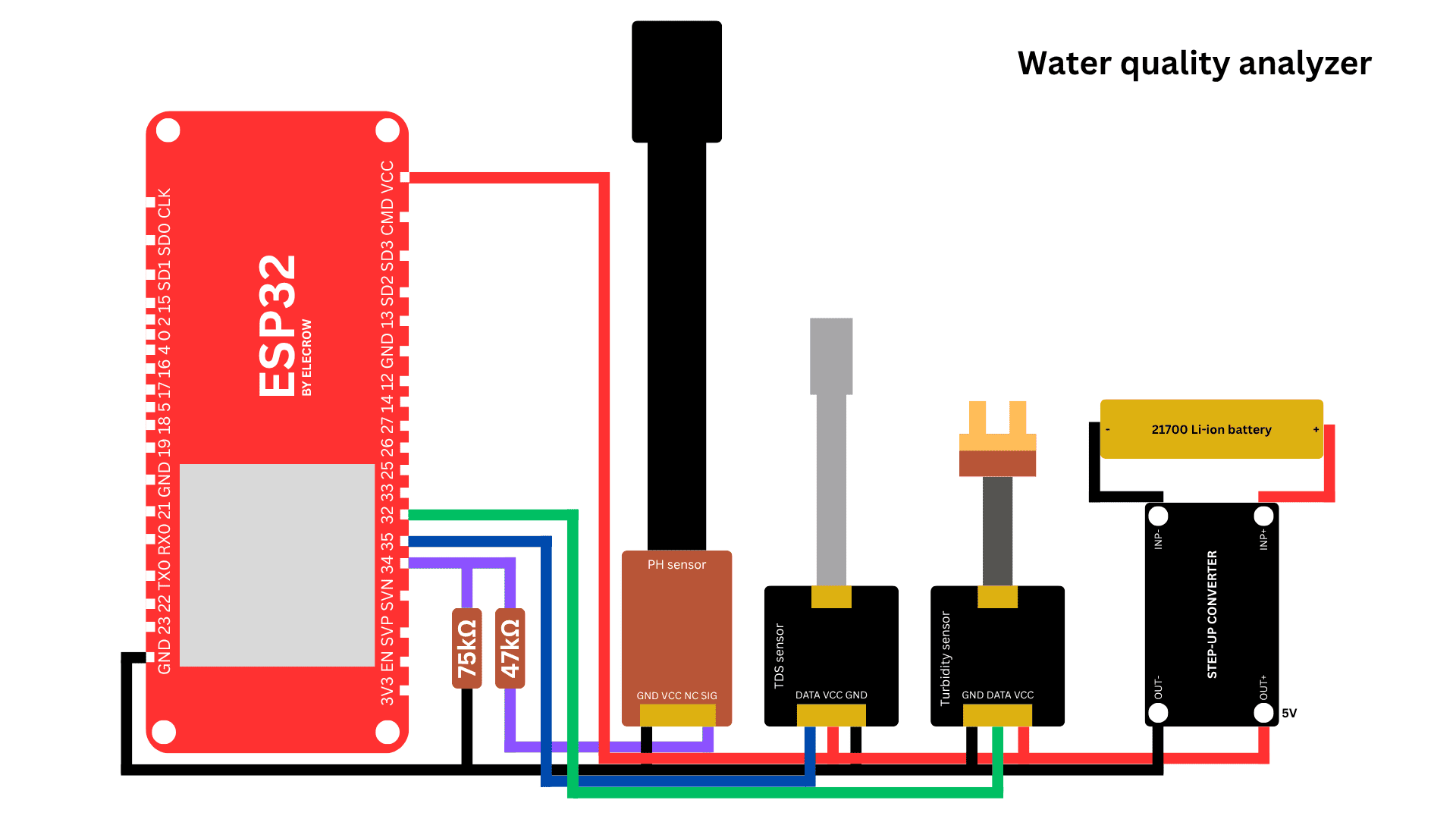
Circuit Assembly and WiringThe hardware for this project is relatively straightforward and can be assembled on a breadboard in a few minutes.
Start by placing the ESP32 on the breadboard and connecting the power rails. Since all sensors in this project operate from a 5V supply, I used a step-up converter powered by a single 21700 lithium-ion battery.
Before connecting any sensors, adjust the output of the step-up converter to 5V using a multimeter. This step is important because supplying an incorrect voltage can damage the sensor modules or produce unreliable measurements.
Once the power supply is ready, the sensors can be connected to the ESP32.
PH Sensor
The pH sensor is connected to GPIO 34 through a voltage divider made from a 47kΩ resistor and a 75kΩ resistor.
This voltage divider is necessary because the pH module used in this project can output voltages close to 5V, while ESP32 analog inputs are designed for much lower voltages.
The divider reduces the sensor output to a safe level before it reaches the microcontroller.
Connections:
- pH signal output → 47kΩ resistor
- Junction between resistors → GPIO 34
- 75kΩ resistor → Ground
If your pH module already outputs voltages within the ESP32 input range, the voltage divider can be omitted.
TDS Sensor
The TDS sensor requires only a single analog input connection.
Connections:
- Signal output → GPIO 35
- VCC → 5V
- GND → Ground
Turbidity Sensor
The turbidity sensor is connected in a similar manner.
Connections:
- Signal output → GPIO 32
- VCC → 5V
- GND → Ground
Final Connections
After wiring all three sensors, connect the ESP32 to the power rails and attach the battery.
If everything has been connected correctly, all modules should power up immediately. There's a schematic below in case you need additional help to wire the components.
At this point, the hardware assembly is complete and the project is ready for calibration.
This project was sponsored by Elecrow.
Elecrow is a supplier of open-source hardware, development boards, electronic components, and manufacturing services for makers, students, and engineers.
In addition to ESP32 development boards, they offer services such as PCB fabrication, PCB assembly, CNC machining, and custom manufacturing.
I've used several of their products in previous projects and have generally been impressed by the build quality and reliability.
If you're looking for components or manufacturing services for your next electronics project, they're worth checking out.
Their support helped make this project possible.
Sensor CalibrationCalibration is one of the most important steps in this entire project.
The sensors used here do not directly output meaningful engineering units. Instead, they generate analog voltages that must be translated into pH and TDS values through calibration.
Skipping this step can easily produce measurements that are inaccurate or completely misleading.
PH Sensor Calibration
The pH sensor was calibrated using three standard buffer solutions:
- pH 4
- pH 7
- pH 10
For each solution, I immersed the probe and recorded the stabilized output voltage.
The measured values were approximately:
PH   |   VOLTAGE
4    |   1.193 V
7    |   1.053 V
10   |   0.939 V
One interesting observation was that the sensor voltage decreased as the pH increased.
When I plotted the calibration points, they formed an almost perfectly linear relationship. Because of that, a simple linear equation was sufficient to convert voltage into pH:
pH = mV + bWhere:
- V is the measured voltage
- m is the slope
- b is the offset
Using the calibration measurements, I calculated:
- Slope = -23.6
- Offset = 32.2
These values were then added directly to the software and are used every time the ESP32 calculates a pH reading.
TDS Sensor Calibration
The TDS sensor was calibrated using a standard conductivity solution rated at 1413 µS/cm.
Unlike the pH probe, the goal here was to determine a conversion factor between the measured voltage and the known conductivity value.
After measuring the sensor output, I calculated a scale factor that converts voltage into conductivity.
The software then estimates Total Dissolved Solids (TDS) using the common approximation:
TDS = Conductivity * 0.5While this relationship varies depending on the composition of the dissolved substances, it provides a reasonable estimate for general freshwater analysis.
Why Calibration Matters
Many hobby projects skip calibration entirely and simply display raw sensor values.
The problem is that two identical sensors rarely produce identical outputs. Manufacturing tolerances, probe aging, temperature, and environmental conditions all influence the measurements.
Calibration compensates for these variations and allows the analyzer to produce readings that are much closer to reality.
Once both sensors have been calibrated, the ESP32 has everything it needs to begin analyzing water samples.
With the hardware assembled and the sensors calibrated, the next step is uploading the firmware to the ESP32.
The complete source code for this project is available on GitHub. After downloading the sketch (water-quality-analyzer.ino), open it in the Arduino IDE, select your ESP32 board, and upload the code.
Once the ESP32 boots, it begins reading all three sensors and prints the measurements to the Serial Monitor every few seconds.
Although the sketch is relatively short, several important processing steps take place before a final water quality classification is generated.
Sensor Pin Configuration
At the beginning of the code, the analog input pins are assigned to each sensor.
const int PH_PIN = 34;
const int TDS_PIN = 35;
const int TURBIDITY_PIN = 32;
These GPIOs are connected to the ESP32's ADC peripheral and are used to measure the analog voltages produced by the sensors.
The sketch also defines the ADC reference voltage and resolution.
const float ADC_VREF = 3.3;
const int ADC_RESOLUTION = 4095;
Since the ESP32 uses a 12-bit ADC, the analog readings range from 0 to 4095.
Noise Reduction Through Averaging
One common issue with analog sensors is measurement noise.
Electrical interference, ADC imperfections, and sensor instability can all cause readings to fluctuate from sample to sample.
To reduce this effect, the sketch averages twenty measurements before performing any calculations.
int readADC(int pin) {
  long sum = 0;

  for (int i = 0; i < NUM_SAMPLES; i++) {
    sum += analogRead(pin);
    delay(10);
  }

  return sum / NUM_SAMPLES;
}
Inside this function, twenty ADC readings (this value is defined by NUM_SAMPLES) are collected and added together.
The average value is then returned instead of a single raw measurement.
This simple filtering technique significantly improves stability and makes the displayed readings much easier to interpret.
Converting ADC Counts Into Voltage
The ESP32 ADC does not directly report voltage. Instead, it returns a digital value between 0 and 4095.
To convert this number into volts, the sketch uses the following function:
float adcToVoltage(int adc) {
  return (adc * ADC_VREF) / ADC_RESOLUTION;
}
This allows the software to work with actual sensor voltages rather than raw ADC counts.
PH Calculation
The pH sensor produces an analog voltage that varies according to the acidity or alkalinity of the solution.
Because the sensor output passes through a voltage divider before reaching the ESP32, the measured voltage must first be corrected.
float phVoltage = adcToVoltage(phADC) * PH_DIVIDER_FACTOR;The divider factor reconstructs the original sensor voltage before calibration is applied.
Once the corrected voltage is known, the software calculates the pH value using the linear equation obtained during calibration:
float pHValue = (PH_SLOPE * phVoltage) + PH_OFFSET;The constants used in this equation were derived from the pH 4, pH 7, and pH 10 buffer solutions discussed earlier.
Finally, the result is limited to the valid pH range: 0 ≤ pH ≤ 14.
This prevents unrealistic values from being displayed if the sensor experiences noise or temporary instability.
Conductivity and TDS Calculation
The TDS module also generates an analog voltage.
After converting the ADC reading into volts, the software estimates conductivity using the calibration factor obtained from the 1413 µS/cm reference solution.
float conductivity_uS = tdsVoltage * EC_SCALE_FACTOR;This produces an estimated conductivity value expressed in microsiemens per centimeter.
The conductivity value is then converted into Total Dissolved Solids:
float tdsPPM = conductivity_uS * TDS_FACTOR;The factor of 0.5 is a commonly used approximation for freshwater measurements.
While laboratory instruments often use more advanced conversion methods, this approach provides a useful estimate for environmental monitoring applications.
Turbidity Measurement
The turbidity sensor is the simplest of the three sensors.
Unlike the pH and TDS probes, no complex calibration equation is required.
The software simply converts the measured ADC value into a voltage and compares it against experimentally determined thresholds.
float turbidityVoltage = adcToVoltage(turbidityADC);Based on the measured voltage, the water is classified as:
- CLEAN
- MODERATE
- POLLUTED
- VERY POLLUTED
Higher voltages correspond to higher turbidity levels.
In other words, a larger voltage indicates that the water contains more suspended particles.
Pollution Scoring System
The most important part of the sketch is the water quality classification algorithm.
Instead of relying on a single sensor, the analyzer combines information from pH, conductivity, and turbidity.
Each parameter contributes to a pollution score.
For example:
- Extreme pH values add several points.
- Elevated TDS levels add additional points.
- High turbidity increases the score further.
The software then calculates a total pollution score and converts it into a final classification (CLEAN, MODERATE, POLLUTED, and VERY POLLUTED).
This approach is intentionally simple.
The goal is not to replicate laboratory-grade analysis but rather to combine multiple indicators into a single, easy-to-understand result.
Serial Monitor Output
Every two seconds the ESP32 prints a complete report.
The report includes:
- Raw ADC values
- Sensor voltages
- Estimated pH
- Conductivity
- TDS concentration
- Turbidity level
- Final water quality classification
Displaying both the raw and processed measurements makes troubleshooting much easier because you can immediately determine whether a problem originates from the sensor hardware or from the conversion equations.
Collecting Water SamplesWith the analyzer fully assembled and calibrated, it was time to see how it performed outside the workshop.
For this test, I collected water samples from two rivers located within a large urban area. Although both waterways pass through residential neighborhoods, they are not connected to each other, making them interesting candidates for comparison.
Before collecting any samples, I spent some time observing the surrounding environment. While the analyzer can provide useful measurements, visual inspection often reveals clues that sensors alone cannot capture.
River #1
The first river appeared relatively shallow and surprisingly clear.
In several areas, I could easily see the riverbed through the water. At first glance, it looked cleaner than I expected.
However, a closer look revealed several signs of human activity. Houses were located near the riverbanks, and small amounts of trash were scattered throughout the area.
What caught my attention most were a few pipes discharging some kind of liquid directly into the river.
I couldn't determine what was flowing through them, and I have no evidence that the discharge was harmful. Nevertheless, seeing unidentified liquids entering a waterway is always concerning.
After documenting the location and spending a few minutes observing the surroundings, I collected a sample using a clean plastic bottle and moved on to the second site.
River #2
The second river created a very different first impression.
Unlike the first location, the area was surrounded by much denser vegetation. There was less visible trash, and I didn't notice any obvious discharge pipes or signs of industrial activity.
At first glance, it appeared to be the healthier of the two locations.
However, a few details stood out.
The water looked noticeably murkier, and there was a persistent unpleasant odor near the riverbank.
Another observation was more subjective but equally interesting: the area felt unusually quiet.
I didn't notice birds, insects, fish, or other obvious signs of wildlife activity. While this alone doesn't prove anything, the lack of visible animal life was difficult to ignore.
After collecting the second sample, I returned home and prepared both samples for testing.
The following day, I used the analyzer to evaluate both water samples.
As with any hobby-grade environmental monitoring project, it's important to remember that these measurements should be viewed as indicators rather than definitive scientific conclusions. Professional laboratory testing would be required to verify the exact water chemistry.
Even so, the results were quite revealing.
Results - sample #1
The first sample was collected from the river where I observed the suspicious discharge pipes.
After allowing the readings to stabilize, the analyzer classified the sample as: POLLUTED.
The most surprising measurement was the pH value.
The sensor reported a pH of approximately 12.7, which is extremely alkaline. For comparison, many household cleaning products fall within a similar range.
Natural freshwater systems typically do not exhibit pH values anywhere near this level. When unusually high pH values are observed, they can sometimes be associated with industrial contamination, chemical runoff, or improper waste disposal.
The conductivity measurement was relatively low, suggesting that the concentration of dissolved ions was not particularly high.
Meanwhile, the turbidity sensor indicated fairly clear water.
This result highlighted one of the main reasons for combining multiple sensors. Although the water appeared visually clean, the pH reading suggested that something unusual might be occurring chemically.
During testing, I also discovered an error in my turbidity classification thresholds. The sensor was initially classifying clearer water as dirtier than it actually was.
After identifying the problem, I corrected the thresholds in the software and repeated the analysis.
Results - sample #2
The second sample produced a surprisingly similar outcome.
The analyzer again reported a pH value close to 13, indicating extremely alkaline conditions.
Conductivity remained relatively low and was broadly consistent with the measurements obtained from the first river.
The main difference appeared in the turbidity reading.
The turbidity voltage increased to approximately 0.8V, indicating a significantly larger concentration of suspended particles.
Unlike the first sample, this result matched what I observed visually. The water appeared murkier, and the sensor confirmed that observation.
The analyzer once again classified the sample as: POLLUTED
Interpreting the MeasurementsAt first glance, the results might seem contradictory.
Both rivers exhibited unusually high pH values, yet neither sample showed exceptionally high conductivity.
Several explanations are possible.
The sensors themselves may have limitations that affect measurement accuracy.
Environmental conditions may also influence the readings.
Another possibility is that the rivers genuinely contain alkaline contaminants that do not significantly increase conductivity.
Without laboratory testing, it is impossible to determine which explanation is correct.
What can be said is that both rivers displayed characteristics that warrant further investigation.
One location contained visible trash and suspicious discharges. The other exhibited murky water, an unpleasant odor, and a notable absence of visible wildlife.
The sensor data alone cannot prove that either river is polluted. However, when combined with direct observations from the field, the results paint a picture that is difficult to dismiss.
Lessons Learned
One of the most valuable outcomes of this project was learning how easily visual observations can be misleading.
The first river looked relatively clean but produced some of the most unusual measurements.
The second river looked dirtier, and the turbidity sensor confirmed that assessment, but the conductivity measurements suggested a more nuanced situation.
This is exactly why environmental monitoring often relies on multiple measurement methods rather than a single test.
No individual sensor tells the whole story.
By combining pH, conductivity, turbidity measurements, and direct field observations, it becomes possible to build a much more complete understanding of water quality than any single indicator could provide on its own.
Failed AttemptsWhat makes this project slightly unusual is that the breadboard prototype you're seeing here was never supposed to be the final version.
My original goal was to build a fully portable water quality analyzer that could be taken directly into the field.
The plan included:
A custom PCB
- A custom PCB
- A 7-inch touchscreen display
- A dedicated enclosure
- Integrated PCB for all sensors
On paper, it sounded like a great idea.
In practice, it became a reminder that engineering projects rarely go exactly as planned.
The Enclosure Problems
One of the first issues appeared during the enclosure design process.
I created a custom 3D-printed enclosure intended to hold the display, electronics, battery, and sensors in a single portable package.
Unfortunately, several design mistakes slipped through the initial review.
The internal dimensions were tighter than expected, cable routing was difficult, and installing the display turned out to be far more challenging than anticipated.
What looked perfectly reasonable in CAD software became much less practical once physical parts were sitting on the workbench.
After several attempts to make everything fit, it became clear that forcing the design forward would create more problems than it solved.
The PCB Failure
The enclosure wasn't the only setback.
I also designed a custom PCB specifically for this project.
After assembling the board and performing some initial tests, everything appeared to be working correctly.
Then the board failed.
After troubleshooting the circuit, I eventually discovered the cause.
While designing the PCB, I had accidentally swapped the positive supply and ground connections.
A simple mistake.
The kind of mistake that many engineers, hobbyists, and students make at some point.
Unfortunately, simple mistakes can have expensive consequences, and the board was permanently damaged and had to be abandoned.
A Better Alternative
Although the original PCB failed, the idea of simplifying the wiring still made sense.
Instead of redesigning the entire portable system immediately, I created a smaller shield PCB that allows the sensors to connect directly to an ESP32 without relying on a breadboard and dozens of jumper wires.
The shield dramatically simplifies assembly while preserving the flexibility of the original prototype.
More importantly, it provides a solid foundation for future versions of the analyzer.
Note: This PCB was designed to work with an Elecrow ESP32 board. If you are using an ESP32 from another manufacturer, the pinout may be different. Be sure to check your board's pinout before connecting it on the PCB.
Future ImprovementsAlthough the current analyzer performs well as a proof of concept, there is still plenty of room for improvement.
One of my main goals is to eventually return to the original idea of a fully portable water quality analyzer.
Future versions may include:
- A dedicated enclosure designed specifically for field use
- An integrated display for standalone operation
- GPS logging for geotagged measurements
- Wi-Fi connectivity
- SD card data logging
- Temperature compensation
- Improved calibration procedures
- Additional water quality sensors
I'd also like to compare the analyzer directly against professional laboratory equipment to better understand its accuracy and limitations.
That comparison would provide valuable insight into how useful low-cost environmental monitoring systems can be in real-world applications.
Open-Source FilesThis project is completely open source. The repository contains:
- ESP32 source code
- Wiring information
- Calibration parameters
- PCB design files
- Supporting documentation
Feel free to modify the design, improve the software, adapt it to different sensors, or use it as the foundation for your own environmental monitoring projects.
If you create your own version, I'd be interested to see what improvements you make.
ConclusionThis project started as an attempt to build a low-cost water quality analyzer using an ESP32 and a handful of readily available sensors.
By combining pH, conductivity, and turbidity measurements, the system is able to provide a quick estimate of water quality while remaining affordable and relatively easy to build.
Along the way, the project involved failed PCBs, enclosure redesigns, calibration work, software debugging, and field testing. While not every part of the process went according to plan, each setback helped improve the final result.
The river tests also highlighted an important lesson about environmental monitoring: appearances can be deceptive.
Water that looks clean is not always clean, and water that looks polluted is not always as contaminated as it seems. Meaningful conclusions often require multiple measurements, repeated testing, and careful observation of the surrounding environment.
This analyzer is not intended to replace laboratory equipment, but it demonstrates how inexpensive hardware can be used to investigate real-world environmental questions and gather useful data.
If you're interested in ESP32 development, environmental monitoring, or sensor-based projects in general, I encourage you to build your own version and experiment with it.
You may discover things about your local environment that would otherwise go unnoticed.
And before the leave this article, I recommend you read this another one about RYLR993 Lite LoRa module with Arduino. I'm sure it'll help you take your maker skills to the next level.
Thanks for reading this lesson, and I'll see you in the next one.


_3u05Tpwasz.png?auto=compress%2Cformat&w=40&h=40&fit=fillmax&bg=fff&dpr=2)
Comments