The main objective of this project is to build a robust and reliable 4 DOF (Degrees of Freedom) robotic arm, based on direct current motors. The idea is to develop a platform capable of moving everyday objects such as soda cans, smartphones, small bottles, etc.
Main components of the arm
The movement of each rotational axis is driven by a powerful actuator consisting of a brushed DC gear motor. This configuration allows the prototype to handle a maximum payload of 350 g, with a reach of up to 80 cm. The structure of the robotic arm is made entirely of aluminum and has a total weight of 6.5 kg. A gripper, based on an open-source design, is attached to the third link and is equipped with a RealSense D435 depth camera for manipulation purposes (beyond the scope of this project).
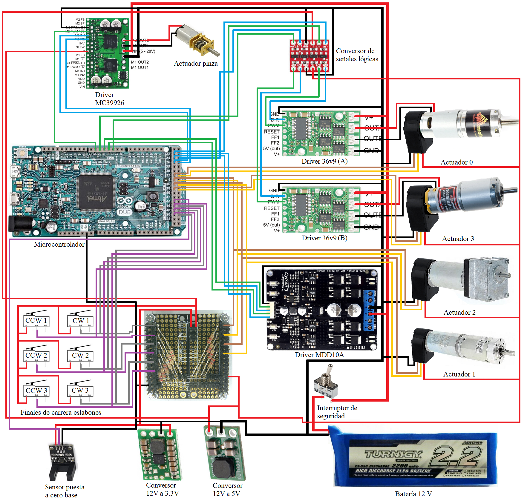
Each of the motors is coupled to a relative encoder that provides information about axes positions and they are powered by its corresponding electronic driver. A 12V battery supply the power for all components of the robot, which has a safety switch that could cut off the power just in case of a possible emergency. The control SW is executed through a powerful 32-bit ARM core processing unit that works at 84 MHz and has a 512 KB memory (Arduino Due board) to store the different computer programs.
The device has been built entirely from scratch. This fact provides a high level of knowledge about the device, their components, and their design decisions. Multiple programming tasks have been developed, oriented both to the control of the different motors and to the kinematic models that correspond to a higher level of control.
PROJECT STEPS
1. MOTORS SELECTION & HW DESIGN
Correct selection of actuators is an important part of the designing any robotic device. These components are responsible for generating the movements and forces required to carry out the tasks for which the robot is designed. In our case, the requirements are 0.35kg of payload and 0.8m maximum range.
Diagram used for calculating the maximum torque required
Taking as a reference, the maximum torque required for each motor is calculated taking into account not only the maximum range and payload but also the weight of the structure of the robot itself as well as the other motors. For that reason, the first calculus correspond to the motor 3, which able to add that weight to the motor 2 calculus. Referring to the actuator 0, on the base axis, the calculus was made using friction forces. The needed torque in each axe is shown below for development purposes:
Motor 0: 8.3 Nm; Motor 1: 8.8 Nm; Motor 2: 3.3 Nm ; Motor 3: 1.0 Nm
Once all motors are selected, the mechanical design can start. It's important to take into consideration the durability of the mechanical connections and the forces that will apply in each movement over the time in order to design a sturdy links.
CAD design process
2. BUILDING THE ARM
Ordering to machining the aluminum parts might be expensive for some so, I recommend you buying a 3mm thick aluminum sheet and do it yourself. You can later join the pieces using inexpensive aluminum tubes, which are also easy to cut and machine. To makes things easier, you can paint the aluminum and engrave with a laser machine all the lines to be cut.
building the robot
Another piece of advice is to make a layout of all the electronic devices which are going to be mounted inside the base of the robot before drilling the mounting holes. This action should be made in order to reduce the amount and length of the electrical connections. In the next image I show you my distribution but you can choose whatever meets your needs.
robotic arm base layout
Usually, the encoders which are supplied mounted in the actuators are relative ones. For sure, depends on your budget. If it is your case, you can transform this relative info about the position of each link into an absolute one. All you need is limit switches for detect the mechanical limits and a simple initialization algorithm. Things are a little bit complicated for the rotation axe of the base but you can also make it with and optical switch like shown below:
1 / 2 • optical switch
3. SW DEVELOPMENT
First of all, a coordinate reference system must be created. This references will be used later for the initialization algorithm and finally for kinematics and the control SW. An example of this reference system could be the next one:
maximum ranges and reference system
Second, we need to have referenced all the axes with their limits, in other words, absolute positions in each degree of freedom. From this information it will be possible to develop closed-loop control algorithms, essential in a device with these characteristics. To obtain the data about the position in an absolute way, the initialization algorithm described below has been developed using the limit switches integrated in the prototype.
Initialization algorithm phases
The initialization algorithm starts from an initial resting position. This is a passive configuration in which no actuator consumes battery power, since the only force acting on the links—gravity—is supported by the robot's own structure. Next, the four actuators of the arm rotate in the directions indicated in Figure B. These directions are chosen to keep the center of mass close to the geometric center of the arm, thereby maintaining the stability of the assembly during the initialization process. Speed profiles were designed for each link to ensure a stable and continuous velocity throughout all phases of initialization. In this way, high accelerations are minimized when the links approach their physical limits or change direction.
An interrupt service routine (ISR) is programmed for each link and is executed when the corresponding limit switch is activated. A priori, the total number of pulses emitted by the encoders over their full range of motion is known. With this information, when the ISR is triggered upon reaching the known physical limit, it becomes possible to establish an absolute position. The initialization process for each actuator is carried out independently. Once the physical limit is reached, the links move to their midpoint, thereby returning to the original neutral position.
Another important task for developing higher levels of control is to design and tune the control system for each link. A PID controller (Proportional, Integral, Derivative) has been implemented—one of the simplest types of controllers and a common example used in engineering schools to teach basic control techniques. This controller operates based on the error, which is defined as the difference between the desired command and the real-time value of the system variable. In this case, the goal is to manage the position error of the actuators.
actuators control architecture diagram
Taking into consideration the specifications of each actuator (see the component information) and the variables used in the code, you can use the data related to the constants of all the PID controllers I have as a reference for your development. You can find this information in the code repository attached to the hackster project.
At this point we already have full control of each link individually. But, a robotic arm is intended to use as a manipulator so it is necessary to calculate and compute its kinematics. This step will allow us to impose control commands over the end effector (gripper) position and speed over time (trajectories). I recommend you to calculate the direct and inverse kinematics by yourself in order to understand the process, mathematical tools and physical implications behind, to become a good robotics engineer.
A practical approach to obtaining the forward kinematics is the Denavit–Hartenberg (DH) method. You can refer to the following paper as a guide to ensure correct implementation: DOI: 10.1109/ICCAR.2015.7166008. Ultimately, this process will allow you to derive the equations that relate the position coordinates and the orientation (around just one axis of rotation, remember we have only 4 DoF) of the gripper to the angular positions of each joint (the configuration space, q). This is known as direct or forward kinematics. For reference, I have provided the solutions below, where the lX variables represent the lengths of each link:
Finally, to make possible the control of the position of the gripper you will have to calculate the inverse kinematics. With the previous equations you only can know where the gripper is in the Cartesian space and its orientation. The practical variable to work with in order to control the arm is the speed/position of each joint. By this way, and with the low level PID controllers he have already implemented, our robotic arm will just work like a charm!
To compute the inverse kinematics I have implemented the Inverse Jacobian method. You can google it to better understand but basically uses the following strategy to reach the desired equations:
diff(pe)=J*diff(q) -> diff(q)=J^-1*diff(pe)
I recommend you to test and check the derivatives of the Jacobian matrix and all the algorithm in general before to code it into the micro-controller. For that purpose I created a Matlab script which is included into the Github code repository, it is called as 'BRAZO.m'. You can find in this file also the solutions of all the equations you need to implemented the inverse jacobian algorithm. Using the built in algebra and plot Matlab methods it is so much easier and faster to check if there is any bug or math error.
Example of linear movement testing from the Matlab file
4. TEST AND ENJOY!
Once you’ve successfully implemented the code into your micro-controller, it’s time to test it and enjoy the results of all your hard work.
initialization and inverse kinematics testing
Also you can use this arm to create more complicated systems like the mobile manipulator shown in the next video.
Red and black lines represent power supply, brown and yellow ones are for the encoders A and B channel signals, blue refer the CW and CCW directions, green the PWMs (speeds), grey and purple for the limit switches. signal


Comments