


Hardware components | ||||||
 |
| × | 1 | |||
 |
| × | 1 | |||
 |
| × | 1 | |||
 |
| × | 3 | |||
 |
| × | 1 | |||
| × | 1 | ||||
 |
| × | 1 | |||
| × | 1 | ||||
| × | 1 | ||||
 |
| × | 1 | |||
 |
| × | 1 | |||
| × | 1 | ||||
| × | 20 | ||||
Software apps and online services | ||||||
| ||||||
 |
| |||||
 |
| |||||
 |
| |||||
Hand tools and fabrication machines | ||||||
 |
| |||||
 |
| |||||
 |
| |||||
 |
| |||||
 |
| |||||
 |
| |||||
 |
| |||||
 |
| |||||
In Kerala alone, a single water contamination crisis led to 31,536 Hepatitis A cases and 82 deaths. This disaster highlights a systemic flaw: community water sources are almost never tested proactively.
A prime example is the Ambedkar Colony well in Varapetty, where residents continued drinking water that was 100% positive for bacterial contamination (MPN) and showed unsafe pH drops to 5.71 simply because it looked clean and had never been regularly tested.
Under the current system, water sampling happens only after dozens of local residents fall severely ill and flood hospitals. This reactive approach effectively turns ordinary people into human test subjects, forcing them to suffer preventable health crises before contamination is ever officially acknowledged and addressed.
Field SurveyField Survey Report: Muvattupuzha River Stretch & Ambedkar Colony (Varapetty)
Our field survey evaluated water quality across public drinking sources, focusing on the Thommankuthu-to-Thennathoor stretch of the Kaliyar-Muvattupuzha River and an adjacent community well at Ambedkar Colony. Physical sampling and laboratory testing across both locations yielded critical data:
100% Pathogen Contamination: Laboratory culture tests confirmed positive MPN (Most Probable Number) counts across all sample points along the river stretch and the Ambedkar Colony well, proving widespread coliform bacterial contamination.
Chemical Oxygen Demand (COD) Spikes: River and well samples consistently exceeded permissible COD safety limits, confirming heavy organic pollution that renders the water unfit for public consumption without treatment.
Acidic pH Drift: On-site digital meter logs recorded unsafe acidic drops down to 5.71 in community source samples.
Seasonal Degradation: Comparative analysis revealed reduced water quality indices (WQI) during dry flow periods, concentrating pollutants in sources used daily by residents.
Our survey highlighted a critical systemic risk: because the water appeared clear to the naked eye, local families consumed it daily, completely unaware of its toxic baseline. Because traditional lab testing requires manual collection, transport, and days of processing, these sources were left unmonitored—proving that current testing models flag contamination only after people drink and fall ill.
Thelima is an Arduino UNO Q based water Quality score calculator which uses Sensor Fusion to combine 4 water parameters: pH, TDS,Turbidity,Temperature and runs a Anomaly detection model to generate the score (it says how much the water have deviated from the healthy stage)
This scores are then send to the local representative (ward member) so he can take actions like testing water, chlorination if the contamination level exceeds
The implementation is done by using a processing unit and a Buoy
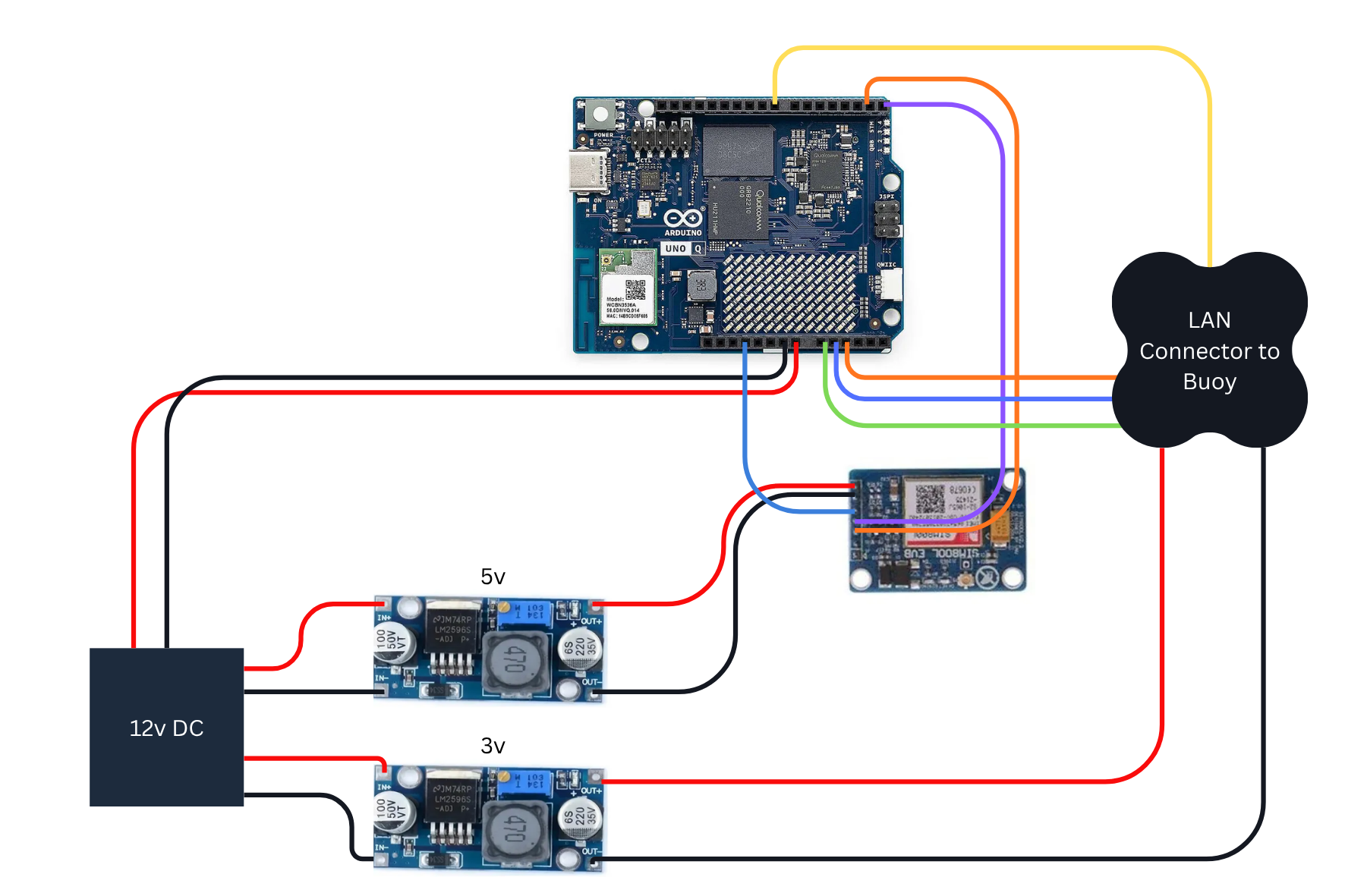
The buoy houses the sensnors and basic voltage divider circuits accurately measuring the above mentioned parameters and sends the values to the processing unit [Arduino UNO Q] through a LAN cabel
SMS send to the public representative Phone:
Getting the junction box ready!
For building the processing unit i am taking a solar junction box with a transparent lid , you can consider any enclosures available to you
Drilling Slots and inserting the connectors and cable groomets
Currently i am having 4 Entry/Exit points and i am using industrial level LAN couplers and groomets for relaibility , a simple hole is also is an option while building primitivly
The connects are ready!
Setting the Electronic Boards
The next step is setting up the platform (Skeleton ) insode the box, The STL files for the 3d printed parts are attached below
Setting up the 3D printed parts
Stacking
The Top and base are connected using M3 sharp screws
The Structure is Ready now lets Insert the electronics Layer by layer as i have mention in the starting of this session
Power Layer
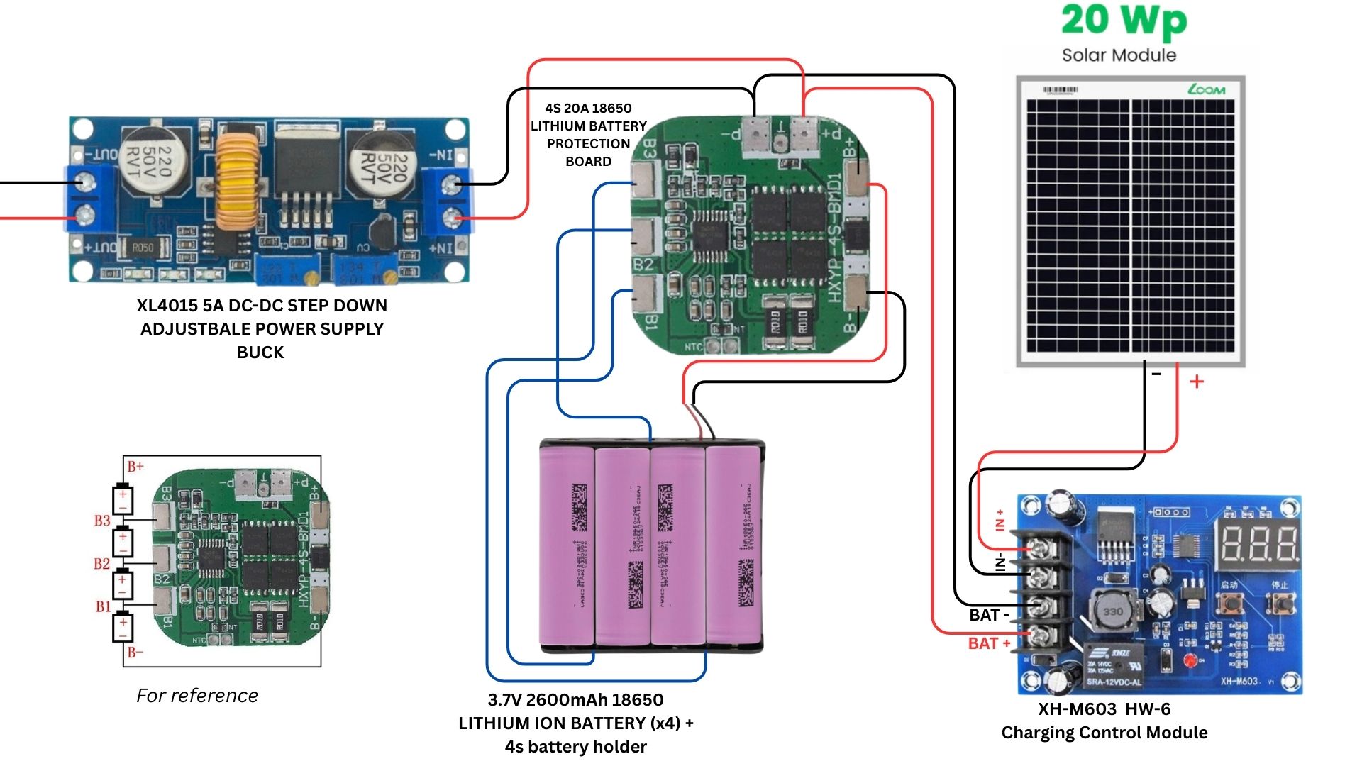
Setting up the 4s 3.7v Li-ion Cell setup powers the circuit in situations of now power or when the live supply is interupted
Setting Up the 5v and 3.3v Rails and fixing it to the skeleton
Here i am using Buck converters , others ways are using UNO Qs own power(not reccomended for long uses)
The Rails are inputted either from the External DC or from the on-board Battery pack!
You Can refer the given circuit diagrams for wiring up the circuit
Making the Power DB + LAN Coupler
Use the provided circuit diagram to implement the power DB and LAN interfacing board, here i have done it on a zero PCB , a OG PCB is the best option. I am also add a Capacitor of 1000uF parallel to the 5v rail to meet the power requirements for the GSM 800L V2 modules
This boards gives power to all on board electronics and sending power to the sensor bouy also gets the sensor data from the buoy
Attaching the DB board to the skeleton
Attaching the LAN Cabel
Setting up the Solar Charge controller Board
Here i am mounting the board above the Power DB board using M3 nut and bolt ladder method , Also
i am routing the 2core wire for the 20W solar panel which keeps the cycles working ;check image 2
Setting Up the Communication Layer (GSM on 3G/2G)
The board uses a GSM chip to send the Health score and adress to the Local representative so that he can act upon any contaminations, the UFL antenna connects to this board
The power terminals the (VCC, GND ) is connected using a screw terminal to reduce the resistance and issues caused buy jumpers at time of instant current
Completion of the Communication Layer
Placing the mighty ARDUINO UNO Q
The final step that is remaining for the unit is adding the ARDUINO UNO Q which acts as the central processing unit which
1)Takes the input from the sensor bouy
2)Process and finds the anomaly score (Using K Means Clusturing)
3)Send the Health score to the Local Rep on GSM communication
Finishing Up the connections and inserting the skeleton into the Junction BOX
insert video here
Assembling the 3d printed parts:The respective models can be found attached on the project
Inserting the sensors and water proofing using Fevi-Seal (silicon tube) :
The sensors are inserted on respective slots and are fixed in place using this silicon which also prevents water from getting inside
Sealing:
The sensors are now fixed in place , Let it dry for 30-40 mins
its will take 2-3 Hr to fully be water proof
Next Step is integrating the Electronics inside and connecting it to the LAN Couplng board
Lets Wire the sensors to the coupling board as per the schematic
Cabel managing and connecting the Lan connector
Attaching the Support Hook : This hook acts as a holding point while we dip the buoy in deep wells
Looping Rope for hanging
The buoy is ready to be deployed!
Step 1 — Create and name the project
1. Sign in at <https://studio.edgeimpulse.com> and open your profile page
2. Click **Create new project**.
3. Enter the project name — e.g. water-quality-node.
4. Choose the project type: **Personal** (60 min job limit, 4 GB / 4 h of data) is enough for
this workload. **Enterprise** removes job and data limits.
5. Choose the project setting: **Public** (anyone can view/clone under the 3-Clause BSD license)
or **Private** (free accounts get a limited number of private projects).
6. Click **Create new project**.
The new project appears in your project list and opens in Studio.
Step 2 — Open the project dashboard and confirm the data
Open the project and check the **Dashboard**. It shows the data collected / imported,
the train-test split, and the project info. Confirm here that:
· the **training set contains only normal samples**, and
· the **test set contains both normal and abnormal samples**.
3b. Processing block
Step 1 — Click Add a processing block → Flatten.
Step 2 — Why Flatten. It reduces each window to a few summary statistics per axis (average, min, max, RMS, standard deviation). The fault signal here lives in the level and trend of the readings, not in frequency content — at 1 Hz there is no oscillation for a spectral block to analyse. Flatten is also the cheapest block (~1 ms, 608 B RAM), which matters on constrained hardware.
Step 3 — Note the output size. 4 axes × 5 statistics = 20 features per window; that is what the learning block receives.
3c. Learning block
Step 1 — Click Add a learning block → Anomaly Detection (K-means).
Step 2 — Why K-means, not a classifier. A classifier needs labelled examples of every fault; you only have reliable examples of normal water. K-means learns where normal data sits in the 20-feature space and flags anything far from it — so it also catches fault types never seen in training.
Step 3 — Check the wiring. Input: the 20 Flatten features. Output: a single anomaly score (distance from the nearest learned cluster). No class labels are produced — that's why model testing later talks about anomaly / no anomaly instead of sensor_fouling.
Step 4 — Click Save Impulse.
Step 4 — Configure the Flatten block parameters
Open **Impulse design → Flatten → Parameters**.
· **Scale axes:** 1 (no rescaling of the raw values)
· **Method:** enable Average, Minimum, Maximum, Root-mean square, Standard deviation
With 4 axes × 5 statistics this produces 20 features per window. The right-hand panel shows
the DSP result for the selected sample plus the on-device cost — here **1 ms processing time**
and **608 bytes peak RAM**, which is why Flatten is a good fit for constrained hardware.
Click **Save parameters**; Studio moves you to the *Generate features* tab.
Step 5 — Generate features
Step 1 — Open Flatten → Generate features in the left menu (Studio takes you here automatically after saving the Flatten parameters).
Step 2 — Click Generate features. Studio slices every training sample into 28.8 s windows using the 6 s stride, runs the Flatten DSP block over each window, and stores the resulting 20 features (4 axes × 5 statistics) as the training matrix. This is a job — it runs on the server and streams a log.
Step 3 — Wait for the job to finish and read the summary. For this project it reports:
Training set: 3h 4m 48s of data
- Training set: 3h 4m 48s of data
1,540 training windows generated
- 1,540 training windows generated
1 class — normal (correct: anomaly detection must be trained only on normal behaviour; if any abnormal class appears here, the data split is wrong — fix it in Data acquisition and re-run)
- 1 class —
normal(correct: anomaly detection must be trained only on normal behaviour; if any abnormal class appears here, the data split is wrong — fix it in Data acquisition and re-run)
Normalization: scikit-learn StandardScaler — each feature is rescaled to zero mean and unit variance so that axes with large numeric ranges (e.g. tds_mgl) don't dominate the K-means distance over small-range axes (e.g. ph)
- Normalization: scikit-learn
StandardScaler— each feature is rescaled to zero mean and unit variance so that axes with large numeric ranges (e.g.tds_mgl) don't dominate the K-means distance over small-range axes (e.g.ph)
Step 4 — Check the Feature explorer on the right. It plots the 1,540 windows in reduced dimensions. You want the normal data to form one or a few tight groups — that is the shape K-means will wrap clusters around in the next step. Widely scattered points mean the windows are too noisy or the window size is too short.
The **Feature explorer** on the right plots the windows in reduced dimensions. For anomaly
detection you want to see the normal data forming one or a few tight clusters — that is what
K-means will model.
Step 6 — Configure the anomaly detection block
Open **Impulse design → Anomaly detection**.
7. **Cluster count:** 32.
More clusters = a tighter envelope around normal data (more sensitive, risk of
over-fitting); fewer clusters = a looser envelope (fewer false positives, risk of missing
subtle anomalies). 32 is a good starting point for a few thousand windows.
8. **Axes:** select the input features the model should use. Click **Select suggested axes**
to let Studio pick the most informative ones, or tick them manually — for this project the
Flatten outputs of all four sensors (ph, turbidity_ntu, tds_mgl, temp_c:
average / minimum / maximum / RMS / stdev) are used.
Step 7 — Train the model
Click **Save & train**. The training output panel streams the job log.
Wait for **Job completed (success)**. Training K-means on this dataset takes well under a minute.
Step 8 — Inspect the anomaly explorer
Still on the anomaly detection page, scroll to the **Anomaly explorer**. Use the dropdown to
switch between training data and individual test samples.
Selecting the test sample sensor_fouling.010 gives:
· Minimum anomaly score: **4.3924**
· Maximum anomaly score: **45.0210**
· Average anomaly score: **31.1626**
Normal windows sit inside the learned clusters and score low; abnormal windows sit far from
every cluster centroid and score high. Use these numbers to pick your **anomaly threshold**:
a value comfortably above the maximum score seen on normal data and below the typical score
of abnormal data. (Scores are unitless distances — always calibrate them on your own data.)
Step 9 — Test the model on the held-out test set
Open **Model testing**. The table lists every test sample with its expected outcome.
Click **Classify all**. Studio generates features for the test files and runs the model over them.
Step 1 — Read the per-sample columns. Each row now shows an anomaly score and a result such as 20 anomaly. The number is not a severity — it is how many windows inside that sample were flagged. A 5-minute sample sliced at a 6 s stride contains ~50 windows, so 20 anomaly means 20 of them fell outside every learned cluster.
Step 2 — Expect N/A for accuracy and the confusion matrix. The anomaly block only knows two outcomes, anomaly and no anomaly. Your test samples are labelled with descriptive class names (sensor_fouling, rain, sensor_drift, …), so Studio cannot match prediction against expectation and scores nothing. This is a labelling mismatch, not a failed model.
Step 3 — (Optional) Get a scored confusion matrix. Open the ⋮ menu on each test sample, set its expected outcome to anomaly (for fouling, drift, contamination) or no anomaly (for normal), then re-run Classify all. Accuracy and the matrix now populate.
Step 4 — Judge the model on the scores, either way. The meaningful signal is the separation: abnormal samples (fouling, drift) score high, normal samples score low. Use the gap between the highest normal score and the lowest abnormal score to set the anomaly threshold you'll apply on-device — pick a value inside that gap. If the two ranges overlap, raise the cluster count or lengthen the window rather than trusting the threshold.
Step 10 — Deploy and build the .eim
9. Open **Deployment**.
10. Click the **Deployment target** box and type linux in the search field. Every entry whose
description says *"An EIM binary … that implements the Edge Impulse Linux protocol"* produces
an .eim: *Linux (AARCH64)*, *Linux (ARMv7)*, *Linux (x86)*, *macOS (arm64/x86)*, the
Qualcomm/BrainChip/TI accelerated variants, and — used here — **Arduino UNO Q**.
Targets like *Arduino library* or *C++ library* produce **source archives, not an .eim**.
Pick the one matching your board's CPU architecture.
11. Click **Build**. The build output panel streams the cross-compilation log.
12. When the build finishes you get a **"Built <target> model"** dialog and the browser
**downloads the .eim automatically**. If it does not, re-download it by clicking the build
name under **Latest build** (e.g. v6 (Arduino UNO Q)) — that link is the download URL
printed at the end of the build log
(https://studio.edgeimpulse.com/v1/api/1105586/deployment/<version>/download).
Past builds are listed under **Latest build → View all deployments**.
The downloaded file for this project:
water-quality-node-linux-aarch64-v6-impulse-#1.eim (~4.9 MB)
The name encodes project, architecture, build version and impulse number.
Step 11 — Use and preserve the .eim
The .eim is a self-contained executable: DSP block + trained model in one file.
Move the downloaded file into your project (e.g. a models/ folder) and make it executable.
- Move the downloaded file into your project (e.g. a
models/folder) and make it executable.
Test it with the Edge Impulse Linux runner before wiring it into your app.
- Test it with the Edge Impulse Linux runner before wiring it into your app.
Call it from your application (Python/Node runner), feeding one 28.8 s window at a time with the axes in impulse order, and compare the returned anomaly score against the threshold chosen in Step 8.
- Call it from your application (Python/Node runner), feeding one 28.8 s window at a time with the axes in impulse order, and compare the returned anomaly score against the threshold chosen in Step 8.
Keep it in version control and note the build version (v6) and impulse number.
- Keep it in version control and note the build version (
v6) and impulse number.
Rebuild whenever you retrain the impulse or move to a different CPU architecture — the binary is aarch64-only.
- Rebuild whenever you retrain the impulse or move to a different CPU architecture — the binary is
aarch64-only.
Step 1 — Connect and select your board. Launch Arduino App Lab. On the Welcome to Arduino App Lab screen, pick your board (here pasu — Arduino UNO Q) connected via USB or over the network. [Image: welcome-select-board.png]
Step 2 — Open the Apps workspace. Once the board connects, App Lab opens the Apps view listing the apps already on the board (e.g. Water Quality AI, WQI Calculator). [Image: apps-workspace.png]
Step 3 — Start the import. Click Create new app + at the top right and choose Import App from the dropdown. [Image: import-app-menu.png]
Step 4 — Upload the app package. In the Import an App dialog, drag and drop your app onto the drop zone, or click Import from computer. Only .zip files are supported. [Image: import-dialog.png]
Step 5 — Pick the file. Browse to the folder holding your exported app (e.g. Documents\hack2026), select the .zip (here WaterQualityAI.zip) and click Open. [Image: file-picker.png]
Step 6 — Verify. App Lab adds the app to your workspace along with its files, Bricks and libraries. The new card appears in the Apps list — open it and press Run to launch it on the board; the status bar shows the running app name with a Stop button.
Tip: the .zip must be an App Lab project export (app files + Bricks), not a bare sketch folder — otherwise the import is rejected.
Future PlansMulti-node deployment with a shared gateway to localise anomalies
- Multi-node deployment with a shared gateway to localise anomalies
Classify the fault type, not just detect it
- Classify the fault type, not just detect it
Self-calibrating thresholds per site
- Self-calibrating thresholds per site
Solar + LoRaWAN for remote, unattended nodes
- Solar + LoRaWAN for remote, unattended nodes
Cloud dashboard with SMS/Telegram alerts
- Cloud dashboard with SMS/Telegram alerts
Add dissolved oxygen and nitrate sensing
- Add dissolved oxygen and nitrate sensing


Comments