Making the control

Published December 30, 2018 © GPL3+

Make Controls with MEGA 2560 - Part 4: The Heater Control

Part 4 is about the theoretical model and the way it is implemented in the AFSM.

IntermediateProtip4 hours993

Make Controls with MEGA 2560 - Part 4: The Heater Control

Things used in this project

Hardware components

Arduino Mega 2560

Story

This part (Part 4) is about the way a Finite State Machine is implemented in the AFSM software. First some theory:For short, a finite state machine consists of states and transitions. A state consists of actions to be performed in that specific state. An example of an action could be the running state of a motor or an active loop for keeping a certain level in a tank. So the first thing to do, is to divide the machine in states, called “finite states”. To go from one state to another, transitions have to be made. A transition consists of one or more conditions and the actual transition to the new state (or states) to go to, when the conditions are true. It is possible to go to one or more states from the active state, depending on the number of defined transitions.

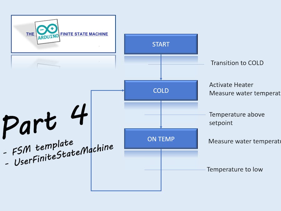
The FSM is best described by an example. "The water heater control". The water heater control is a very simple control for holding the temperature on a certain temperature. See the figure below for the theoretical model:

Theoretical model of the heater control

The states are named in the rectangles with a short description. The actions performed in the states could be described in a matrix (up to you). In this particulary case the actions are so simple, that i've writen them next to the state. Transistion between states are drawn with arrows. The line crossing the arrows describe the condition to make a transition.

Some design philosophy: When starting the control, always the "Start" state is the first and only state to be active. All other states are initially "hibernating" and will not be executed in the loop. In the start state all I/O can be examined and a transition to the right state(s) can be made to initially start the control. This is done because it is never known in what sort of state the "field" is, during the start. Another detail concerning the digital output (DO) datapoints: a DO can be activated in an active state (e.g. a pump, valve). When not activated in a state, the digital output datapoint will be not activated. Deactivation of a DO is not necassery.

The short description of the heater control; When started, there is an immidiate transition to the COLD state; presume the water is in all cases to cold. In the COLD state, activate the HEATER and measure the water temperature (TTWATER). When the temperature is higher then the high setpoint for the temperature, make a transition to state ON TEMP. In the ON TEMP state, measure the temperature TTWATER. When TTWATER is colder then the lower setpoint, make a transition to the COLD state. The endless loop is made.....

Making the control

For the definition of the control, 2 files have to be adjusted. Both part of the sketch; UserConfiguration.h and UserStateMachine.h.

Header files

The UserConfiguration.h contains the declarations of the datapoints (defined by the Configurator) and the declaration of the states. For the heater control, 2 states have to be added to the alraedy existing START and END state; COLD, ON-TEMP.

Add states

Edit the UserConfiguration.h file and load the sketch to the board. When starting the HMI, you will get already the complete set of states. Active states, are "checked" in the list. At this moment only the Start state is checked, the default state to start.

New states added

Now the control can be made in the UserFiniteStateMachine.h file. First the common structure of a state. First of all there is the header with the state name, then between brackets the functionality, consisting of 4 logical parts (order is important, but not every part is necassery).

The Enter state action.This code is run just one time when entering th state. Could be usefull for debug actions; e.g. print to the serial monitor that the state is entered.
The State functions. It is an open door; but when this is an active state, this code is run in an endless loop. In our example, the activation of the HEATER in the COLD state.
The Transition conditions.The conditions and the transistion to other state(s). You can make transistions to one or multiple states. These states will become active. Keep in mind; when making a transition from a caller state, the caller state will leave the active states and is not run in the next cycle (the state is going into hibernation, unless you make a transition to the caller state itself, pfffff....). If you make a transition to the END state, the caller state will go into hibernation, whitout activating another state. When just one state is active, a call to the END state, will kill the control (game over). See also the explanation on the website.
The Exit state action. Just like the enter state action; but than when leaving the state.

To make the writing of transiton conditions easier, there are predefined functions available. e.g. the boolean function DigRising("SWITCH"). You can find these functions on the website. Below the code for the START state.

START state

In the COLD state, the HEATER has to be activated and the tempearature TTWATER is measured. Lets say that a temperture of higher than 24 degrees is condition for jumping to state ON-TEMP and a temperature of 22 degrees is the condition to get the HEATER on again. I simple hysteresis of 2 degrees. Build and load the sketch.

COLD and ON-TEMP state.

And than the final test, take a watercooker, a DS18B20 temperature sensor and a relay. The result (.... in dutch we say: a control with an overshoot where a horse gets the hiccups of...)

Pen plotter Heater control

This is just a very simple example of a control made by/with the AFSM software.
There is no more editing needed than posted in this project; this is the greatest benefit of using the standard AFSM environment (i think...) . You can find much more information and examples of controls on my website www.jbsiemonsma.nl.
In part 5 the digital pen plotter will be explained in detail.

User Finite State Machine

// UserFiniteStateMachine.h

//*========================================================================================
//*  Application code
//*
//*  Name: UserFSM()
//*  Version:
//*  Date:
//*  Author:
//*
//*  Short description:
//*
//*
//*========================================================================================
//*========================================================================================
//*============ START USER APPLICATION ======= START USER APPLICATION =====================
//*========================================================================================
//*========================================================================================
//
// State machine
//
// Each phase exists of 2 parts, e.g. the phase actions and transition conditions.
// In the phase actions, all activated tags are mentioned. Deactivation is not needed, deactivation is
// done at the end of the main loop. In the conditions section, all conditions for the transitions to another
// phase are mentioned. When all condition are true, the new phase can be set. It is possible to programm
// more then 1 transition. In such a case it is necassery to keep the priority in mind.
//
//*========================================================================================


void UserFSM()
{
	//
	// Machine state "START" is the default state at 
	// startup of the board!
	//
	if (MachineState == FiniteState("START"))
	{
		//Enter state action
		if (EnterState()) Serial.println("START state is entered");

		// The state function
		// No actions to perform is this state.
		
		// Transaction conditions
		TransitionToState("COLD");	

		//Exit state action
		if (ExitState()) Serial.println("START state is exit");

	};


	if (MachineState == FiniteState("COLD"))
	{
		//Enter state action
		if (EnterState()) Serial.println("COLD state is entered");

		// The state function
		Activate("HEATER");

		// Transaction conditions
		if (TempValue("TTWATER") > 35.0) TransitionToState("ON-TEMP");
		
		//Exit state action
		if (ExitState()) Serial.println("COLD state is exit");
	};


	if (MachineState == FiniteState("ON-TEMP"))
	{
		//Enter state action
		if (EnterState()) Serial.println("ON-TEMP state is entered");

		// The state function
		// No action required in the state

		// Transaction conditions
		if (TempValue("TTWATER") < 34.0) TransitionToState("COLD");

		//Exit state action
		if (ExitState()) Serial.println("ON-TEMP state is exit");
	};



	//*========================================================================================
	//*========================================================================================
	//*============  END USER APPLICATION ========= END USER APPLICATION =====================
	//*========================================================================================
	//*========================================================================================
}

Credits

Jelle

8 projects • 19 followers

I'am developing software only during rainy days.

Make Controls with MEGA 2560 - Part 4: The Heater Control

Things used in this project

Hardware components

Story

Making the control

Code

User Finite State Machine

Credits

Jelle

Comments

Embed the widget on your own site

Make Controls with MEGA 2560 - Part 4: The Heater Control

Make Controls with MEGA 2560 - Part 4: The Heater Control

Things used in this project

Hardware components

Story

Making the control

Code

User Finite State Machine

Credits

Jelle

Comments

Related channels and tags