

Hardware components | ||||||
| × | 1 | ||||
| × | 1 | ||||
| × | 1 | ||||
 |
| × | 1 | |||
Software apps and online services | ||||||
| ||||||
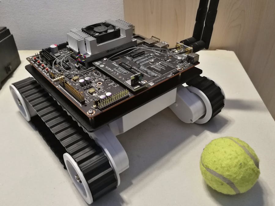
I have started a project to explore machine vision APIs in Nvidia TX1. I am able to capture camera stream from onboard 5 MP Fixed Focus MIPI CSI Camera in OpenVX and track any object within it. The next part is to integrate it with a Rover so that it can follow an object if it starts to move away.
I will continue to post update here as I make progress. Stay tuned!
BackgroundI am using this project as a learning exercise for computer vision. Below I'll discuss the different approaches that I tried to find and track the tennis ball, with a discussion of their strengths, weaknesses and lessons learned. I will start with the basics and work my way up from there.
I prototyped my algorithms in Octave, which is an Open Source Matlab equivalent.
Template Matching
Here we have the scene on the left and template on the right. We need to implement software that can identify the rectangle in the scene where it finds the template
One way of doing is with normalized Correlation. We will need to do some pre-processing to get there. First step is to convert it to grey scale by eliminating the hue and saturation information while retaining the luminance.
scene = imread('scene.jpg');
pkg load image
scene_grey = rgb2gray(scene);
template = imread('template.jpg');
template_grey = rgb2gray(template);
Before running the correlation operation I needed to resize the image to keep computation cost under control.
template_gr = imresize(template_grey,0.1);
scene_gr = imresize(scene_grey,0.1);
c = normxcorr2(template_gr, scene_gr);
figure, surf(c), shading flat
There is no prominent peak in this. It did not find the match. Our tennis ball template has a texture and it is not just a plain circle. The detailed texture will never map exactly, unless it was cut from the same image. Lets try Gaussian Blur to remove the undesirable details.
template_grs = imsmooth(template_gr, 'Gaussian', 2.00);
scene_grs = imsmooth(scene_gr, 'Gaussian', 2.00);
c = normxcorr2(template_grs, scene_grs);
figure, surf(c), shading flat
figure, imshow(c);
Now you can see the peak in the 3D surface plot. When correlation results is drawn as image, you can clearly see the bright white spot where the match was found.
This is great, but it does not work well when ball is moving and its distance from camera changes. Variable lighting and occlusion can easily throw this algorithms off.
Feature detection
In previous section we learned that we can find the ball by looking at raw pixels and try to find a match or correlation, but this scheme does not work will with real world images captured from varying distance under different lighting conditions.
Alternative to comparing raw pixels, we can try to find the tennis ball by its characteristics. Let us examine the image by plotting it as intensity map:
figure, surf(double(scene_grs)), shading flat
The tennis ball shows as a steep cliff with round top. Now we can use some established techniques to detect this 'feature'. Notice how that z axis goes from 0 to 250. The reason is that a grey-scale png image uses a single byte to represent one pixel and hence it can only represent 2^8 = 256 levels.
- Edge Detection
How do we detect a steep cliff with round top? Image can be considered as a mathematical function f(x, y). We are are looking for steep changes in that function. Generally speaking, we want to covert an image which is f(x, y) into a reduced set of pixels or curves that captures the important elements of image somehow such that we only deal with the changes that matter.
In mathematical functions change is about Derivatives.
The Derivatives here can also called gradient, which is a vector since typically we would have change in both x and y. The magnitude of gradient tells how quickly things change and the direction where there is most rapid change in intensity.
The calculations happens i two steps: 1) Apply filter that returns image gradient function. 2) Threshold the gradient function to find edge pixels.
There are lot of well known operators that can be used find gradient function. The following are implemented in Octave.
sobel = fspecial('sobel')
sobel =
  1   2   1
  0   0   0
 -1  -2  -1
prewitt = fspecial('prewitt')
prewitt =
  1   1   1
  0   0   0
 -1  -1  -1
outim = imfilter(double(scene_gr),sobel);
imagesc(outim);
colormap gray;
outim_p = imfilter(double(scene_gr),prewitt);
figure, imagesc(outim_p);
colormap gray;
- Thresholding
Octave has builtin function to compute gradient. The default method is 'sobel'. Lets experiment with different thresholding values.
[g_mag,g_dir] = imgradient(scene_grs);
threshold = 20;
g_mag_t = g_mag .* (g_mag >= threshold);
figure, imshow(g_mag_t/8)
The divide by 8 is done to normalize the output of 'sobel'. Please see this.
As you can notice, as threshold value goes up, small details and noise goes away and we are left with only significant details. Please note that we are only dealing with gradient magnitude, the direction will come into play later.
Octave has built-in support for the sobel edge detection. In fact you can get a result similar to above with the following:
edge_sobel = edge(scene_gr,'sobel',0.031214, 'both', 'nothinning' );
If you look at lower right of the Tennis ball, you will notice two things, the edge is many pixel thick, it can be fixed by a technique known is 'Non-Maximum Suppression'.
edge_sobel = edge(scene_gr,'sobel,0.031214,'both', 'thinning');
Again if you look at lower right corner you will notice that some pixels did not survive the thresholding. This topic is subject of research for many decades. One way to fix this is to use Canny's method and performs threshold hysteresis.
edge_canny = edge(scene_grs,'canny',0.2);
Its better but still not perfect. Considering the fact that we know Tennis Ball is round, which make a close shape. It so happens that 'Laplacian of Gaussian' edge detector with a threshold of zero will detect close contours s because it includes all the zero-crossings in the input image.
It detected the round Tennis ball but also added lot of false edges. All of the above need to be fed to a higher level algorithm to find circle shape that best represents the Tennis ball.
- Hough Transform
Hough transform has been around for a long time and it attempts to solve the problem of extracting structure from an Image. Essentially we go from pixels to things. In our case the structure is the circle created by the edges of Tennis ball. The older view of looking at computer vision was to look at the edges and and try to find analytic models like lines and circles. Modern approach is to detect templates which serve as a visual code words to describe a feature.
[centers, radii, metric] = imfindcircles(scene_gr,[30 50]); % Matlab
imshow(scene_gr);
viscircles(centers, radii,'EdgeColor','b');
I had to experiment a little with the radius parameter but in the end It worked well. There are some known limitations of Hough Transform like its time complexity and robustness against noise. I will continue to explore more optimum methods to solve our problem.
This write-up is work in progress.
HardwareRover 5
I received mine as a gift for this project. The Rover 5 tracked chassis, made by Dagu Electronics, is a robot platform with caterpillar treads that let it drive over many types of surfaces and uneven terrain. The chassis features a rugged white plastic body with room to house a battery holder and some additional electronics. Mine has 2 DC motors with 86.8:1 gearboxes, which makes it strong enough to lift the weight of the chassis and allow it to achieve speeds as high as 10 in/s (25 cm/s).
Mine came without quadrature encoders. Since this is a computer vision project so I might be able to get away with using camera to keep track of rover's movement.
Adafruit Motor Shield
I happened to have an Adafruit Motor Shield already in my collection. Although it is made for an Audrino, I think I can re-purpose it to interface with Nvidia TX1 and the Rover 5.
This shield handles all the motor and speed controls over I2C. Only two data pins, SDA & SCL in addition to the power pins GND & 5V are required. Given its I2C, I can make it talk to Nvidia TX1. The only issue is that this Shield uses 5V logic levels while Nvidia TX1 is 3.3V. I am using Four Channel Level Converter to solve the voltage issue. I could get away with 2 channel level converter because I2C is 2 channel protocol, but the 4 channel variant was already in my collection.
This boasts TB6612 MOSFET drivers with 1.2A per channel current capability. You can draw up to 3A peak for approx 20ms at a time. I measured Rover 5 nominal running current per motor to be around 300mA. The stall current is 2.5A. This could work as long as I don't let the motors stall for too long. I am planning to put a seat sink just in case.
This write-up is work in progress.


Comments