
Hardware components | ||||||
 |
| × | 1 | |||
| × | 1 | ||||
 |
| × | 1 | |||
| × | 1 | ||||
| × | 1 | ||||
Software apps and online services | ||||||
 |
| |||||
This project is the final project of SE423 at UIUC.
The goal of this project is to let the robot car navigate through a built track while avoiding the random obstacle in its way. There are several major components of this project.
- Control the robot car and use dead reckoning to get the pose of the robot car
- Process Lidar reading with F28379D Launchpad
- Use Lidar to recognize the obstacle
- Use A* algorithm to find the path
- Communicate with the motion tracking system to navigate through the path
We used the enhanced Quadrature Encoder Pulse (eQEP) peripheral of the F28379D launchpad to get the angles of the motors used in our robot car. With that, it is easy to get the velocity of the robot car with the sample time and the distance traveled. We then used a PI controller to steer the robot car around. Ideally, we can then calculate the pose of the robot car by dead reckoning assuming there's no slip between the wheels and the floor.
Process Lidar dataFor this project, a cheap YDLidar X2 model works well. It can sense a range of 0.10 to 8.0m with a 360° perspective. One great thing about this Lidar is that it will automatically start to collect data the instant it is powered on.
The Lidar can transmit data through the serial port. In this project, SCID is used to accept the data, and the data of the Lidar comes in through pin 9 of the launchpad.
I used an 8-state state machine to interpret and store the Lidar data. The resulting data is in the form of an array with 360 entries, each entry contains the distance and timestamp information of the points detected by the Lidar, and the index of this array is the angle at which the data is collected.
A Detailed explanation on reading the Lidar data can be found at https://www.hackster.io/yixiaol2/using-ydlidar-with-ti-tms320f28379d-6b62c5
Use Lidar to detect obstaclesAfter getting the Lidar data from the last step, we get the information of what the robot sees: the robot is at the center, and there is a distance that corresponds to all integer angles from 0 to 359°. Therefore, a polar plot will be adequate for us to visualize the results.
In our project, we built a 12*12 feet track in the mechatronics lab for the robot car to run within, and the obstacles are wood blocks that are 2*2 feet that can only be placed at the integer grid in the track.
This setup greatly simplifies our obstacle-finding procedure: based on the collected data, we can get the "global view" of the track by coordinate transformation given the initial conditions of the robot car (pose_x, pose_y, pose_theta). Then, round the readings of the obstacle within the range of the track should be adequate for us to get the edge of the obstacle since the obstacle can only appear on integer grids. The following initial condition corresponds to the second figure above, where pose_x is -4, pose_y is 6, and the pose_theta is 30°.
//initial condition
double pose_x = -4; //x_position of the robot car
double pose_y = 6; //x_position of the robot car
//need to put negative initial angle because the Lidar is rotating CW
double pose_theta = 0; //angle of robot car
double pose_rad; //angle in rad
The coordinate transformation is done in the while loop inside the main function. A ping-pong buffer is used to make sure there's enough time to process all the data. In the following code, I first loop through all the points in the buffer array. If the obstacle within 0.1 m of the lidar, which is not detectable by the Lidar thus having a distance of 0, I put it at the origin, which corresponds to the origin globally.
if (pingpts[i].distance ==0) {
        x_f[i].distance = 0;
        y_f[i].distance = 0;
        x_f[i].timestamp = pingpts[i].timestamp;
        y_f[i].timestamp = pingpts[i].timestamp;
}
Otherwise, I first convert the polar coordinate to Cartesian coordinate, and used the change of basis equation to get the "global" position of the detected points. x_ori and y_ori are the direct results from changing polar coordinate to Cartesian coordinate, while x_f and y_f are the final results by change basis and translation.
else {
        x_ori[i] = pingpts[i].distance*cos(i*0.01745329);//0.017453292519943 is pi/180
        y_ori[i] = pingpts[i].distance*sin(i*0.01745329);
        x_f[i].distance = (x_ori[i])*cos(pose_rad)+(y_ori[i])*sin(pose_rad)+pose_x; //change basis
        y_f[i].distance = -(x_ori[i])*sin(pose_rad)+(y_ori[i])*cos(pose_rad)+pose_y; //change basis
Finally, with simple criteria of only considering the obstacle within the range of x:(-6,6), y:(0,12), we can mark the location with points detected as obstacle 'x' on the mapCourseStart array. The mapCourseStart is an array of characters with 176 (11*16) elements that store the map of the track's grid crossing. It contains all '0' during initialization, which means there are no obstacles yet.
char mapCourseStart[176] =      //16x11
{   '0', '0', '0', '0', '0', '0', '0', '0', '0', '0', '0',
    '0', '0', '0', '0', '0', '0', '0', '0', '0', '0', '0',
    '0', '0', '0', '0', '0', '0', '0', '0', '0', '0', '0',
    '0', '0', '0', '0', '0', '0', '0', '0', '0', '0', '0',
    '0', '0', '0', '0', '0', '0', '0', '0', '0', '0', '0',
    '0', '0', '0', '0', '0', '0', '0', '0', '0', '0', '0',
    '0', '0', '0', '0', '0', '0', '0', '0', '0', '0', '0',
    '0', '0', '0', '0', '0', '0', '0', '0', '0', '0', '0',
    '0', '0', '0', '0', '0', '0', '0', '0', '0', '0', '0',
    '0', '0', '0', '0', '0', '0', '0', '0', '0', '0', '0',
    '0', '0', '0', '0', '0', '0', '0', '0', '0', '0', '0',
    '0', '0', '0', '0', '0', '0', '0', '0', '0', '0', '0',
    '0', '0', '0', '0', '0', '0', '0', '0', '0', '0', '0',
    '0', '0', '0', '0', '0', '0', '0', '0', '0', '0', '0',
    '0', '0', '0', '0', '0', '0', '0', '0', '0', '0', '0',
    '0', '0', '0', '0', '0', '0', '0', '0', '0', '0', '0'   };
Points that are within 1 tile of the robot are not considered as it may be some random data collection error. There's a bijective correspondence between the global position(x, y) of the obstacle to the index of the mapCourseStart array that is given by 11*(11-y)+5-x. Here (x, y) is the position of the lidar reading after coordinate transformation and translation.
// code to process the obstacle
        if ((round(x_f[i].distance) >-6) && (round(x_f[i].distance) <6) ) { // within x range
            if ((round(y_f[i].distance) > 0)&& round(y_f[i].distance) < 12) { //within y range
                if ((fabs(x_f[i].distance-pose_x) > 1) && (fabs(y_f[i].distance-pose_y) > 1)) { //neglect points that are too close to the robot car
                    mapCourseStart[(11*(11-(int)(round(y_f[i].distance))))+5+(int)(round(x_f[i].distance))] = 'x'; //set 'x' at correct location
                }
            }
        }
        x_f[i].timestamp = pingpts[i].timestamp;
        y_f[i].timestamp = pingpts[i].timestamp;
    }
}
Below is a figure overlaying the mapCourseStart array with the grid. The points of the mapCourseStart are at the center of each tile.
Therefore, seeing from the robot at the initial condition of pose_x = -4, pose_y = 6, and the pose_theta = 30°, the points with index 18, 29, 40, 41, 42 should change from '0' to 'x' in the mapCourseStart array.
Checking the result from the expression window of Code Composer Studio for the mapCourseStart array, we get the expected result from our code, with index 18, 29, 40, 41, 42 being an obstacle ('x').
The next step is to use a path planning algorithm to find the path for the robot to go.
Implement A* algorithm with diagonal stepsA* is a path planning algorithm that takes both the traveled distance (g) and the distance from the current point to the destination (heuristic value, h) into account. Then it will choose to go to the point with the smallest g+h value. A more detailed explanation can be found at https://www.redblobgames.com/pathfinding/a-star/introduction.html.
The code from previous semesters only considered moving in the horizontal and vertical direction, and the heuristic value here is the Manhattan distance given by |x1-x2|+|y1-y2|. However, it would be more efficient if we consider diagonal moves. Below is the code that I added to the getNeighbors function of the A* algorithm. To make a diagonal move, we need to make sure the adjacent vertical or horizontal neighbors are reachable. That is, if we want to go to the top-left neighbor, we need to make sure we can travel to both the top and left neighbor.
//top left corner, only can travel when both top and left are reachable
	if ((canTravel(rowCurr - 1, colCurr) == 1) && (canTravel(rowCurr, colCurr - 1) == 1)) {
		if (canTravel(rowCurr - 1, colCurr - 1) == 1) {
			nodeToAdd.row = rowCurr - 1;
			nodeToAdd.col = colCurr - 1;
			neighbors[numNeighbors] = nodeToAdd;
			numNeighbors++;
		}
	}
	//top right, need top and right reachable
	if ((canTravel(rowCurr - 1, colCurr) == 1) && (canTravel(rowCurr, colCurr + 1) == 1)) {
		if (canTravel(rowCurr - 1, colCurr + 1) == 1) {
			nodeToAdd.row = rowCurr - 1;
			nodeToAdd.col = colCurr + 1;
			neighbors[numNeighbors] = nodeToAdd;
			numNeighbors++;
		}
	}
	//bottom left, need bottom and left reachable
	if ((canTravel(rowCurr + 1, colCurr) == 1) && (canTravel(rowCurr, colCurr - 1) == 1)) {
		if (canTravel(rowCurr + 1, colCurr - 1) == 1) {
			nodeToAdd.row = rowCurr + 1;
			nodeToAdd.col = colCurr - 1;
			neighbors[numNeighbors] = nodeToAdd;
			numNeighbors++;
		}
	}
	//bottom right, need bottom and right reachable
	if ((canTravel(rowCurr + 1, colCurr) == 1) && (canTravel(rowCurr, colCurr + 1) == 1)) {
		if (canTravel(rowCurr + 1, colCurr + 1) == 1) {
			nodeToAdd.row = rowCurr + 1;
			nodeToAdd.col = colCurr + 1;
			neighbors[numNeighbors] = nodeToAdd;
			numNeighbors++;
		}
	}
If we can travel diagonally, the heuristic value is closer to the Euclidean distance than the Manhattan distance. Therefore, I updated the heuristic value function and changed all the distance-related values from integer type to double type.
double heuristic(int rowCurr, int colCurr, int rowGoal, int colGoal)
{
	int rowDiff = rowCurr - rowGoal;
	int colDiff = colCurr - colGoal;
	return sqrt(rowDiff * rowDiff + colDiff * colDiff);
}
Lastly, the distance traveled in diagonal is sqrt(2) instead of 1 in the previous vertical and horizontal movement. So I updated the traveled distance calculation.
if (abs(next.row - minDistNode.row) + abs(next.col - minDistNode.col) == 2) {
    next.distTravelFromStart = currDist + sqrt(2);
} else {
    next.distTravelFromStart = currDist + 1;
}
Below are test cases for small, medium, and large map path planning. we can see that traveling diagonally can indeed save some steps (pathLen) and distance traveled (the next.distTravelFromStart value), thus more efficient.
The points from the A* algorithm are tracked in the nodeTrack array, after calling the reconstructPath function, we can get the path that is in pathRow and pathCol in the correct order from the starting point to the ending point.
Navigating from point to point is done through the provided xy_control function. We need to pass the pathRow and pathCol values with the correct index into the function.
We can use dead reckoning to get the pose data of our robot car. However, since the wheel may slip during the operation, there will be some errors with the dead reckoning that may accumulate with time. Therefore, to make sure the robot car performs as expected, we use the Optitrack system set up at mechatronics lab to get a more precise pose of our robot car.
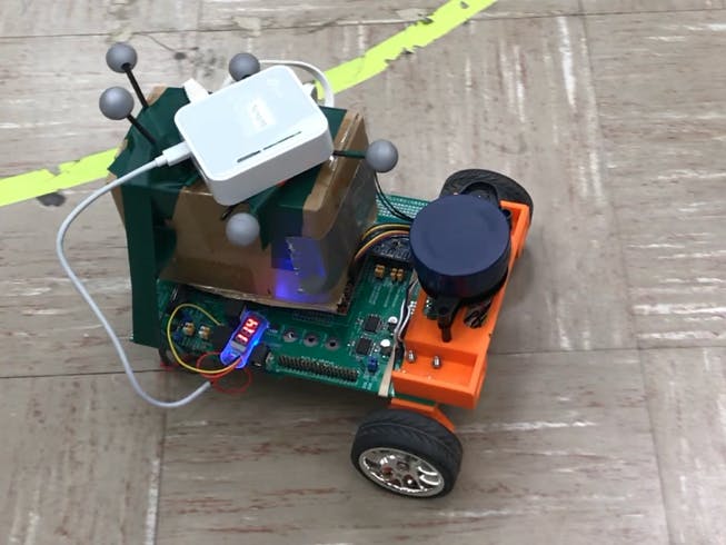
For the Optitrack systems to function, we first need to set the robot car at an angle of 0°, with the robot's coordinate's direction lined up with the global coordinate. After selecting the reflective balls set on the top of the robot car in the Motive software and running the scripts that send the data through the router connected to the lab's computer, we only need to find a way to receive the data. Here I used Wiznet W5500 chip to accomplish this. The W5500 chip is a Hardwired TCP/IP embedded Ethernet controller that enables easier internet connection for embedded systems using SPI (Serial Peripheral Interface).
W5500 is connected to GPIO122, 123, 124, 125, which correspond to pin 12, 13, 17, 18 of the launchpad. For receiving the data, the UDP protocol is used, with the robot car as UDP server and the computer connecting with the Optitrack as UDP client.
The Ethernet converter module I used provided me with the capability of connecting a router to the robot car. Setting the router in client mode (the mode that usually use for devices without wifi function but with an ethernet port) and connecting it to the router that sends out the data in the configuration webpage, the robot car can get the data from the Optitrack system.
To avoid CPU1 of the launchpad from being too busy and messing things up, I used CPU2 in this project to set up the UDP server, receive, and process the data from OptiTrack. Generally, to use CPU2, we first need to make sure the GPIOs used in CPU2 have their ownership set to CPU2 in the initialization of GPIO in CPU1. Here, we need to set GPIO 0, 122, 123, 124's ownership to CPU2 in CPU1's main function.
//wiznet reset
    GPIO_SetupPinMux(0, GPIO_MUX_CPU2, 0);
    GPIO_SetupPinOptions(0, GPIO_OUTPUT, GPIO_PUSHPULL);
    GpioDataRegs.GPASET.bit.GPIO0 = 1;

    GPIO_SetupPinMux(125, GPIO_MUX_CPU2, 0); // wiznet cs
    GPIO_SetupPinOptions(125, GPIO_OUTPUT, GPIO_PUSHPULL); // Make GPIO2 an Output Pin
    GpioDataRegs.GPDSET.bit.GPIO125 = 1; //Initially Set GPIO2/SS High so wiznet is not selected
    GPIO_SetupPinMux(122, GPIO_MUX_CPU2, 6); //SPISIMOC/WIZNET
    GPIO_SetupPinMux(123, GPIO_MUX_CPU2, 6); //SPISOMIC/WIZNET
    GPIO_SetupPinMux(124, GPIO_MUX_CPU2, 6); //SPICLKC/WIZNET
Then we need to set the peripheral that we used to 1 in the DevCfgRegs register. Here we are using SPIC for communicating, therefore we are using CPUSEL6.
EALLOW;
DevCfgRegs.CPUSEL6.bit.SPI_C = 1;
EDIS;
After the basic setup in CPU1, we can safely put all the UDP server code into CPU2's function. I'm using a separate project for CPU2 here.
For the Optitrack data, it is in the form of x, y, theta, rigid body number, and frame count. Those data are 2 bytes each, but we are only receiving 1 byte each time from the client. Therefore, we need to combine the data together for an entire reading. Here I used a union to store a single set of data received from Optitrack, which has a rawData array with the type of uint16_t and a Data array with the type of float.
typedef union optiData_s {
    uint16_t rawData[10];
    float Data[5];
} optiData_t;
Then by combining the received data, we have the raw data in 2 bytes each, and combining those 2 bytes data as a 4 bytes float, we restore the data from Optitrack. Finally, by setting the IPC register to 1 in CPU2, we interrupt CPU1 to receive the data.
recvsize = recvfrom(0, (uint8_t *)buffer, len, recvfrom_ip, &recvfrom_port);
mydata.rawData[0] = buffer[0] | (buffer[1] << 8);
mydata.rawData[1] = buffer[2] | (buffer[3] << 8);
mydata.rawData[2] = buffer[4] | (buffer[5] << 8);
mydata.rawData[3] = buffer[6] | (buffer[7] << 8);
mydata.rawData[4] = buffer[8] | (buffer[9] << 8);
mydata.rawData[5] = buffer[10] | (buffer[11] << 8);
mydata.rawData[6] = buffer[12] | (buffer[13] << 8);
mydata.rawData[7] = buffer[14] | (buffer[15] << 8);
mydata.rawData[8] = buffer[16] | (buffer[17] << 8);
mydata.rawData[9] = buffer[18] | (buffer[19] << 8);
recvcount += 1;
cpu2tocpu1[0] = mydata.Data[0];
cpu2tocpu1[1] = mydata.Data[1];
cpu2tocpu1[2] = mydata.Data[2];
cpu2tocpu1[3] = mydata.Data[3];
cpu2tocpu1[4] = mydata.Data[4];
IpcRegs.IPCSET.bit.IPC0 = 1;
The below figure is the result reading from CPU2.
We then created a float array cpu2tocpu1 for both CPUs to store the data from Optitrack. We then find the location of cpu2tocpu1 ram in the cmd file, setting both to be at the same location in both CPU1 and CPU2, we can then write values to this array in CPU2 and retrieve it in CPU1.
//IPC
__interrupt void CPU2toCPU1IPC0(void){
    GpioDataRegs.GPBTOGGLE.bit.GPIO52 = 1;
    x = cpu2tocpu1[0];
    y = cpu2tocpu1[1];
    theta = cpu2tocpu1[2];
    number = cpu2tocpu1[3];
    framecount = cpu2tocpu1[4];
    OPTITRACKps = UpdateOptitrackStates(ROBOTps);
    ROBOTps.x = OPTITRACKps.x;
    ROBOTps.y = OPTITRACKps.y;
    ROBOTps.theta = OPTITRACKps.theta;
    UARTPrint = 1;
    IpcRegs.IPCACK.bit.IPC0 = 1;
    PieCtrlRegs.PIEACK.all = PIEACK_GROUP1;
}
To run this, we need to first build the project with CPU2, and debug CPU1 project. After CPU1 running, right click on cpu2 and connect target. Under the run menu, load the CPU2.out file. Finally, run CPU1 then CPU2.
Having the Optitrack data, we can use it to command the xy_control function. below is a demo video of the robot car going to several preset points with the motion tracking system telling it its location.
After putting things together, we can let our robot car travel to the destination automatically, avoiding the obstacle.
Below is a video of the robot avoiding obstacles and travel to the desired point.
It also can travel through a small maze.
CreditsThanks to Professor Dan Block for helping me solve all the problems I had during this project and providing essential starter code.
Thanks to TA Hang Cui for the help on UDP communication and the starter code for CPU2,
Thanks to Scott Manhart for designing the Lidar stand.


Comments