

The whole implementation is based on Mariusz's paper Explaining How a Deep Neural Network Trained with End-to-End Learning Steers a Car. This post will discuss the following things:
- Explanation ofthe original paper: How this "Heat Map" works for PilotNet’s model
- ExploreMore: How to design an algorithm that can support all models
- Implement the design supporting customized model
As the name of the paper, it provides a visualization tool to help the user understand what are the "key pixels" in the input image for PilotNet’s model. PilotNet’s model is a 2D CNN model created by NVIDIA which outputs steering angles given images of the road ahead. It's very similar with the default model in Donkey Car platform. Full structure is as follows:
This paper is trying to find the Salient Objects in images of the road ahead, and help engineer to understand how those model works and what impacts the model to make decisions. The approach uses deconvolution to create a mask that can map out those pixels triggering high activations. The process can be defined by the following steps.
Step 1: Average the activations in each layerto get averaged map:
The shape of each activations in each layer will be (1, width, height, channel). To average each layer, we can run following code:
np.mean(activations[layer], axis=3).squeeze(axis=0)
Step 2: Use deconvolution to scale up activations from the top to the bottom
We can use following code to do the deconvolution work. The parameters (filter size and stride) used for the3deconvolution are the same as in the convolutional layer used to generate the map.
       conv = tf.nn.conv2d_transpose(
           x, layers_kernels[layer],
           output_shape=(1,output_shape[0],output_shape[1], 1),
           strides=layers_strides[layer],
           padding='VALID'
       )
As for how conv2d_transpose works, This Link give a very good explanation. I copied the intuition explanation below:
Deconvolution layer is a very unfortunate name and should rather be called a transposed convolutional layer.
Visually, for a transposed convolution with stride one and no padding, we just pad the original input (blue entries) with zeroes (white entries).
Step 3: The up-scaled averaged map from an upper level is then multiplied with the averaged map from the layer below
Step 4: Repeat step 2 & step 3 until reaching to the bottom
Regarding to step 3 and step 4, I will give an explanation on the implementation part.
Design an algorithm that can support all modelsFor some of those self-driving problem, cropping the data from the top or bottom might hep us improve the performance of our model. So before the process of doing convolution, some user will add a crop layer as a pre-process layer. By doing some modifications, we can make the "heat map" algorithm works fine with cropping layer as well.
Original design is only for PilotNet’s model, designing a general algorithm for all models also only needs to change the design in a very minor level.
The full design is as follows:
- Create configuration area
- Load model
- Extract convolution layers and pre-process layers
- Create mask generation algorithm
- Create the output video
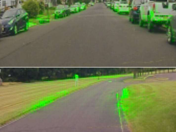
The final "heat map" video looks like this:
ImplementationI have attached full Jupyter code in the coding section, in this section, I will go though the key component.
Create configuration area:
Configuration area is for defining all model specific variables, such as input image shape, pre_process_layers, etc.
# Model path:
model_path = "crop22219"
#Shape of your conv input
conv_shape = (120, 100, 3)
#Shape or original inout
orignal_shape = (120, 160, 3)
# Layers before conv layers
pre_process_layers = 2
# Amount of conv layers
conv_layers = 5
Load Model:
# By calling keras API to load the model
from keras.models import Model, load_model
model= load_model(model_path)
Extract convolution layers and pro-process model:
Following code created a model containing only convolutional layers:
img_in = Input(shape=conv_shape, name='img_in')
x = img_in
x = Convolution2D(24, (5,5), strides=(2,2), activation='relu', name='conv1')(x)
x = Convolution2D(32, (5,5), strides=(2,2), activation='relu', name='conv2')(x)
x = Convolution2D(64, (5,5), strides=(2,2), activation='relu', name='conv3')(x)
x = Convolution2D(64, (3,3), strides=(2,2), activation='relu', name='conv4')(x)
conv_5 = Convolution2D(64, (3,3), strides=(1,1), activation='relu', name='conv5')(x)
convolution_part = Model(inputs=[img_in], outputs=[conv_5])
Load the weights from original model to conv model:
pre = layers[:pre_process_layers]
layers = layers[pre_process_layers:pre_process_layers+conv_layers]
print([i.name  for i in pre])
print([i.name  for i in layers])
for layer_num in ('1', '2', '3', '4', '5'):
   convolution_part.get_layer('conv' + layer_num).set_weights(layers[int(layer_num)-1].get_weights())
Wrap conv model and pre-process model:
from keras import backend as K
from keras.layers import Cropping2D
inp = convolution_part.input

outputs = [layer.output for layer in convolution_part.layers]
functor = K.function([inp], outputs)

# pre-process model:
inp = Input(shape=orignal_shape, name='img_in')
outputs = Cropping2D(cropping=((0,0),(60,0)))(inp)
pre_functor = K.function([inp], outputs)
Create mask generation algorithm
Before starting the implementation of mask generation algorithm, we need to specify some features related with the conv layer, such as the size of the kernel, padding, strides and etc. This should be a part of configuration area, in order to make it easier to understand, I moved it to this part.
kernel_3x3 = tf.constant(np.array([
       [[[1]], [[1]], [[1]]],
       [[[1]], [[1]], [[1]]],
       [[[1]], [[1]], [[1]]]
]), tf.float32)
kernel_5x5 = tf.constant(np.array([
       [[[1]], [[1]], [[1]], [[1]], [[1]]],
       [[[1]], [[1]], [[1]], [[1]], [[1]]],
       [[[1]], [[1]], [[1]], [[1]], [[1]]],
       [[[1]], [[1]], [[1]], [[1]], [[1]]],
       [[[1]], [[1]], [[1]], [[1]], [[1]]]
]), tf.float32)
layers_kernels = {5: kernel_3x3, 4: kernel_3x3, 3: kernel_5x5, 2: kernel_5x5, 1: kernel_5x5}
layers_strides = {5: [1, 1, 1, 1], 4: [1, 2, 2, 1], 3: [1, 2, 2, 1], 2: [1, 2, 2, 1], 1: [1, 2, 2, 1]}
The ollowing code is how to generate the mask for different images:
def compute_visualisation_mask(img):
   # get output of activations from the top of the conv shape will be like [1,w,d,c]
   # c is the numbers of channels
   activations = functor([np.array([img])])

   # shape of the top activation map:
   init_shape = activations[-1].shape[1:3]
   upscaled_activation = np.ones(init_shape)

   # iterate through all conv layers from the top to the bottom
   for layer in [5, 4, 3, 2, 1]:
       # average activation maps shape: [1,w,l,c] -> [w,l]
       # multiply with the average map from previous layer
       averaged_activation = np.mean(activations[layer], axis=3).squeeze(axis=0) * upscaled_activation
       # get the shape for next layer
       output_shape = (activations[layer - 1].shape[1], activations[layer - 1].shape[2])
       # Use deconvolution to scale up activations from the top to the bottom        x = tf.constant(
           np.reshape(averaged_activation, (1,averaged_activation.shape[0],averaged_activation.shape[1],1)),
           tf.float32
       )
       conv = tf.nn.conv2d_transpose(
           x, layers_kernels[layer],
           output_shape=(1,output_shape[0],output_shape[1], 1),
           strides=layers_strides[layer],
           padding='VALID'
       )
       with tf.Session() as session:
           result = session.run(conv)

       upscaled_activation = np.reshape(result, output_shape)

   final_visualisation_mask = upscaled_activation
   # get the final mask
   return (final_visualisation_mask - np.min(final_visualisation_mask))/(np.max(final_visualisation_mask) - np.min(final_visualisation_mask))
Create the output image/video
After having the mask map, the code to find salient-object is relatively easy.
   img = cv2.imread(path)
   img = pre_functor([np.array([img])]).squeeze(axis=0)
   salient_mask = compute_visualisation_mask(img)
   salient_mask_stacked = np.dstack((salient_mask,salient_mask))
   salient_mask_stacked = np.dstack((salient_mask_stacked,salient_mask))


Comments