

In the past 15 years, the use of small fixed wing UAVs has significantly increased. Amateurs RC and drone pilots as much as small professional structures are interested in knowing the performance of their aircrafts but can not all afford wind tunel testing. Thus, there is a need for relevant and reliable experimental protocols providing access to aerodynamics characteristics of small fixed wing UAVs. Simple protocols which would only require Commercial Of The Shelf (COTS) components.
Thus, the ultimate goal of this project is to establish a reliable and repeatable protocol which could be used for small fixed wing UAVs, in order to determine experimentally their actual drag polar with a known accuracy. The drag polar being the corner stone to access several aircraft performances. This protocol relies only on COTS components and can this way be used by small UAV builders whithout acess to wind tunel testing.
To achieve that goal, we will access the drag polar of the well known Easy Glider, a 1800mm beginner RC glider, through a series of semi-autonomous glide tests. From that polar, will be deducted the power curve, the velocities for maximal endurance and maximum range, and the minimum turn radius. Those performances will then be challenged experimentally to confront the experimental polar and the theoretical performances based on it, to the reality.
Aircraft characteristics- Total mass : 1.1 kg
- Wingspann : 1.8m
- Wing Area : 0.33 m^2
Hypotheses :
• During our whole flight sessions, both the pitch angle and the angle of attack should not exceed +- 15°. Thus, we will consider the small angle approximations.
• This small angle approximation also enables to consider that the true airspeed is equal to the pitot airpseed. Indeed, as we fly at low altitude, there is no significant difference in the air density between the air on the ground, and the air midflight. For the geometrical point of view, in the worst case scenario :
Vpitot/Vair = cos(15°) = 0.996 = 1
• The wind is horizontal and steady. Thus, the vertical airspeed is given by the barometer.
1. Principle
Without a proper knowledge of the efficiency of our powertrain, and since this value has been demonstrated by the literature to vary substantially with the airspeed, the option of accessing the polar through semi-autonomous sink tests has been selected.
In those conditions, the Cd is obtained by the power balance between the only two forces working on the aircraft while dead stick : the weight and the drag.
Thus, we have :
Power_of_𝑤𝑒𝑖𝑔ℎ𝑡 = 𝑤𝑒𝑖𝑔ℎ𝑡 ∗𝑉𝑧 = 𝑃ower_of_𝑑𝑟𝑎𝑔 = 0.5∗ ⍴∗𝑆∗𝐶𝑑∗𝑉air^3
=>𝐶𝑑 = (2∗𝑤𝑒𝑖𝑔ℎ𝑡∗𝑉𝑧) / ( ⍴ ∗𝑆∗𝑉air^3)For the CL, as the glider flying almost horizontally, the weight is almost equal to the lift. Thus, we almost have :
CL = (2∗𝑤𝑒𝑖𝑔ℎ𝑡)/( ⍴ ∗𝑆∗𝑉^2)Where S is the wing area provided in the hardware section, V is the airspeed given by the airspeed sensor, Vz the vertical speed given by the barometer, and ⍴ is the air density. The density is computed for every flight analysis with the ideal as law, using the local atmospheric pressure and temperature as an input.
The flight controller Speedybee f405 wing used is flashed with Inav 7.0. This configuration does not enable to fix the airspeed on a sink test. However, playing with the different modes, we can fix a target attitude, which leads the aircraft to reach an equilibrium state. The data can then be recorded once that equilibrium state is reached.
Thus, it was decided to rely directly on the ANGLE MODE from Inav. In that configuration, the pilot directly sends on live the target pitch and bank angles to the flight controller.
2. Programming and set up
The idea is to be able to perform different sink tests at different equilibrium states, to be able to plot Cl = f(Cd). In order to set steady target pitch angles in a consistent way, the pitch angle control is not given by the transmitter’s pitch stick, which has a recoil spring, but by the wheel, which stays in place.
The wheel’s range is divided in 7, and each 7th of the range is assigned to a pitch angle command [5°; 3°; 1°; 0°; -1°; -3°; -5°].
3. Acquisition procedure
The sink test must be performed in steady air without any thermal activity, and ideally, in low wind. The flight sessions are then held within the first two hours of the aeronotical day, or within the last hour of the aeronautical day.
• At the begining of the flight session, the temperature is mesured at the airfield and the atmospheric pressure from the local airport is written down.
• After loading the mission into the flight controller and arming the model, the pilot proceed to the take of in MANUAL MODE.
• Once the clim bis steady and controlled, the pilots flies towards the test area. The aircraft must respect the legal ceiling, but be high enough for an one minute untouched glide high above the obstacles.
• Once the aircraft is at the correct altitude, the pilot sets the wheel to the position designated for the target pitch angle he wants to set for the sink test.
• When ready to proceed, the pilot cuts the motor, gets the aircraft in a straight steady glide, and activates the CONDITION 0.
• The pilot then lets the aircraft glide for at least 30 seconds without providing any input.
• Once the acquisition sequence is over, the pilot retakes control in MANUAL MODE. The pilot can then, when ready, fly the aircraft towards the test area. The last three steps of the procedure are then repeated for the next iterations.
4. Data processing and results
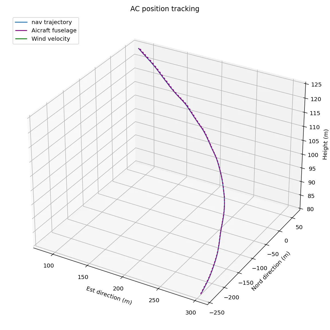
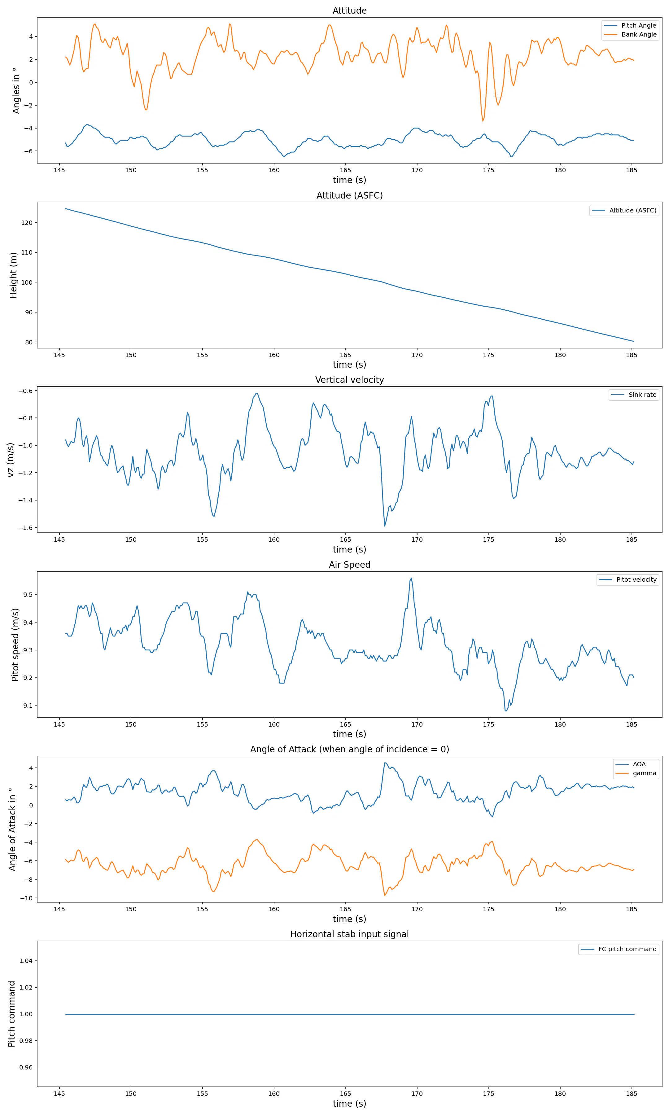
Back in the office, the flight data from the black box are gathered in a CSV file using Inav’s Black box decode tool. The home made Python script is then used to analyse the CSV file and extract the isolate the sink tests, compute and plot, for each sink test, the relevant data. Among other, the Python script requests as an input from the user: the operating temperature, the operating pressure, and the names. As an output, the Python script plots the 3d path of the aircraft on the sequence, evolution of the altitude above surface, evolution of the pitot and vertical speed, evolution of the pitch and bank angles. It also writes in a text file : the operating conditions, the average and standard deviation of the plotted variables, and the resulting values of Cl and Cd. The climb rate angle and angle of attack are also plotted.
After the first flight tests, the experimental results are promising. The campain must still be extended over several flight sessions to get a substantial amount of samples and extract the equation of the polar Cd = f(CL).
08/04/2026:
Since the last update, several flight sessions have taken place. This brings us today to ~40 valid points of mesurements. If all the points have consistent values by themselves, some more need to be taken in order to either draw a solid trend Cd = f(CL) for the polar, or call the experiment inconclusive.
In parallel of the flight test activities, an application coded in Python has been developped to ease the processing of the flight logs, the visualisation and analysis of the experimental results to access the aerodynamic caracteristics of the aircraft, and the aircraft performance prediction based on those caracteristics.
The app App_Aero then has 3 main tabs:
. Library
. Visualisation
. Performance Prediction
Library tab:
In the library, the user can store flight logs, and observe the analyses of the different glides.
When Importing a new flight log, the user enters a name, the operating conditions and import the CSV file of the flight (obtainable from the nativ Inav black box flight log via the INAV Black box decode tool).
When accessing the analysis of a flight log the user can access the detailed analysis of each glide of the session. The app automatically detects the glides, and compute the average vertical velocity and air speeds, the average attitude and angle of attack, and use them to access the CL and the Cd of that point of mesurement. All those values are compelled in a table.
For each glide, the interesting variables usefull to access the values of CL and Cd and those used to evaluate the sability/quality of the glide are also plotted.
Visualisation tab:
In the visualisation tab, the user can visualise the different points of mesurement of the flight logs of his choice, and access the expression of that experimental polar.
Performance prediction tab:
In this tab, the user can see compute the cruise and equilibrated turn performance of its drone. The experimental polar can be used, but the user also has the possibility to use another expression for the polar.
The maximum power deliverable by the powerplan is considered independent of the airspeed, and only depends on the operating pressure.
Thus, this tool is significantly cuts the flight data processing. It is also a dynamic optimisation tool enabling the link the aerodynamics models fed by real world data to an interactive performance prediction wizard.
The next steps of this project are to be carried out on two sides.
.The flight test campaign will be resumed to compile more data and refine the experimental Drag poar.
. In parallel, the work on the development of the application can be continued in order to turn it into either an online tool ,accessible by anyone, or a easily portable format which can be shared and directly used by any user, as the current version relies on Streamlist and requires navigating to the windows terminal.
11/04/2026:
Today, let’s go for flight test. We will try to explore the high angles of attack in priority.
current time: 05:53 am
local sun rise time: 06:28 am
pressure: 1018 hPa
Indicated temperature at the airport: 1°C
indicated wind speed at the airport: 3kts from the sout south south west
eye test:
mesured temperature: 4°C (at the end of the session)
I flew around the end of the last hour of the aeronautical day.
There was a clear blue sky, no cloud visible. Almost no wind feelable. On the anemometer, on the ground, the wind was oscillationg very slowly between 1m/s and 2m/s. In the air, the AC was sometimes stationnary, thus, there was wind, but a very laminar one. My main concern when I arrived was that the sun was rising, and properlly radiating on the country side: I was affraid of thermals. During the flight, I suspected one, but hard to really tell. I also flew alsmost all the time in the same area. After the suspicion of thermal, I tried to do my tests somewhere else. I did around 10~15 glides, trying to explore the middle and middle high points of the polar. The glides seemed of an acceptable stability. I was trying to start the glides with headwind, but it systematically tunred in the tailwind direction at some point. Let’s see how that influences the average bank angle.
According to the blackbox explorer, the flight session lasted for 21 min. At the end I had to land as I had litteraly no more battery at all. After the landing, I noticed a layer of ice on the left wing. Is that due to the landing in the iced grass, or could that be proper icing ??
Let’s see what the flight analysis brings us:
9 glides detected. Overall, they all had a good longitudinal stability: 1% to 4% standard deviation on the TAS, 1°to2° standard deviation of the pitch angle, less that 1° standard deviation on the AOA, 2 exceptions at 34% and 27% (due to transition time to stability) but in general 20% or less standard deviation on the vertical velocity. The main problem concerning the validity of the glides is that there was indeed a significant bank angle (averaging about 4° on multiple glides and sometimes peaking over 10°). This can artificially underestimate my CL and overestimate my Cd.
The analysis of the polar itself tends to confirm that the points I did not really understand from the flight session of the 18/02 are in fact not an exception, but the actual values of the polar. Today, I mainly explored the region I had identified as “problematic” on the 18_02. The pitch angles for the middle high AOAs. Indeed, those have drag coefficients higher than the ones for the smallest AOAs (which is expected), but they have equal or even smaller values of CL, which should not be.
The thing is that the values for the lowest targeted pitch angles and the highest targeted pitch angles, seem to show a logical trend (Cd, and CL rise with the AOA). In green, I drew by hand the kind of polar I would expect especially given the trends set by the extremity. In red, I circled the “problematic points”, which are then probably not an accident since they have been observed on two distinct glides sessions with different conditions.
Could that be due to the high bank angle during those glides ? (artificially increased Cd combined with artificially decrease CL)
The thing is that in that region, on the 18_02_26, there was no significant bank angle. This accidental region is attached to a targeted pitch angle, but not to an actual region of average pitch angle nor an actual region of AOA, nor to a particular airspeed.
Thus, acquiring more data will enable me to have a better vision, and confirm that this is not an accident, but in parallel, the bibliography might help me solve that "mystery".
12/04/2026:
Today, let’s go flying.
current time: 05:32 am
local sun rise time: 06:26 am
pressure: 1013 hPa
Indicated temperature at the airport: 7°C
indicated wind speed at the airport: 4kts from the 210°
eye test:
I arrived at the field and flew at ~07:00
Mesured temperature: 6.6 °C (end of the session)
There was no wind feelable from the ground. There was a low layer of stratus clouds blocking the sun and moving quite fast (from the south west it seemed) : this indicates a proper laminar wind. The clouds were blocking the sun for the whole session, reducing the risk of thermal activity. A little wind was perceptible in flight from the south west, but the contditions were very steady overall: perfect conditons.
I explored points on the neutral position of the wheel, the first and the second higer positions, but ran out of battery before reaching the top position near the stalling point.
4 majors points:
first, on the neutral position, the aircraft kept turning left like yesterday. This default seems to have been better handled by the Flight Controler (FC) for the acquisitions at the upper wheel position. This now definitely needs to be addressed. The default mainly observed for the glides with the wheel around the neutral position. I don’t want to impact physically the AC (not with lateral weight balance nor shape modification) so maybe flight control tuning might be the solution. Increasing the proportional coefficient.
Also critical point, I have noticed that for some glides, the “shut down engine” kept spinning in some sort of idle. Also while in manual with the throttle totally cut off. But this is not systematic. This can have a dramatic impact on the measurement, not that much because of the thrust, but because of the dramatic impact it must have on the drag.
Also, this flight lasted only 17 min. my flight from the 18_02 lasted 45 min. Thus, I will let the battery charge much longer before the next session, and if it keeps coming short, I will have to replace it. The current pulled during the “cut of engine glides” was the same as during the early phase right after the arming of the model. So I am sure that those missed glides are not responsible from the energy shortage.
Also, noticing the parachute trajectory of the glider during the aquisitions for the high AOA points, I thought about questioning one of the primary hypotheses. So far, CL is computed considering that the lift directly balances the weight because cos(glide_path_angle) ~1.
If I now consider cos(glide_path_angle) in my calculations, will that detail correct my polar and reposition properly the accidental points of my polar ?
before changing any of that, let’s see what the flight analysis gives us.
The logs confirm that the bank angle problem was indeed faced for the first glides, those carried out at the neutral position of the wheel.
Once again we are directly in the “problematic “ part. We are getting data which are always more consistent with each other. The points of today and yesterday almost match (we also indeed had very similar conditions). If we can have a few more massive sessions like the one of the 18_02 with 30 points of measurements, we can have a solid an consistent experimental set.
now, let’s try to compute CL differently.
The force balance on the vertical axis gives us:
L*cos(gamma) = Weight
so L = Weight/cos(gamma)
in our case, to compute our CL, we will use gamma = arcsin( Avg_Vz / Avg_Airspeed).
Lets’s see what it changes.
Error detected !!
By rechecking my code, I saw a mistake. Cos(gamma) was indeed used but the line was false:
we were multiplying by cos(gamma) instead of dividing by it.
I corrected the mistake:
The result seems slightly better, but not solved.
15/04/2026:
lert’s go flying.
current time: 05:12 am
local sun rise time: 06:21 am
pressure: 1033 hPa
Indicated temperature at the airport: 3°C
indicated wind speed at the airport: 4kts from the 40° to the 110° (not steady in direction)
Back from the field.
Perfect conditions: no feelable wind, blue sky without cloud, slightly before sun rise, little mist over the surrounding fileds confirming the absence of wind.
Temperature: not taken as the session was aborted shortly.
Indeed, if everything was working perfect on the bench before going, at the moment of assembling the glider on the field, the pin of the airspeed sensor was found broken. So session aborted.
29/04/2026:
I fixed the AC yesterday, today, let’s go flying.
current time: 05:09 am
local sun rise time: 05:48 am
pressure: 1029 hPa
Indicated temperature at the airport: 2°C
indicated wind speed at the airport: 2kts
eye test:
Back from the field. Perfect conditions. Blue sky with a few high contrails. No feelable wind from the ground. This time, I let the battery charge over a night and flight session lasted about 40 min. I explored most of the positions with a high focus on the higher positions of the wheel. All the glides looked clean and steady. Only one glide might be questionable, as for this one, I was flying leveled flight with the motor on and just cut the motor and started the glide without any transition. The AC might then have a high initial airspeed which would not necessarily have had the time to dissipate during the glide. The main problem was that with those perfect conditions, as I arrived the sun was rising (session started probably ~ 6:20am ), and by the end of the 40 min, it had the time to shine. Even the temperature I felt standing on the field seemed higher at the end of the flight that at the beginning. Thus, high risk of thermal activity. Temperature was measured on the field at 3,5°C. Still the same issue with the propeller which might actually not stop entirely. If we are lucky, this might have been the case for all the flights dring the whole campaign.
Let’s see what the flight analysis gives us.
28 glies were detected. They are indeed pretty stable. Standard deviation is usually of about 2% to 3% for the TAS, and of about 10%~15% for the vertical airspeed. One glide has an exceptional deviation of 29% for the vertical airspeed, but we can actually see that the oscillations are high at the beginning but almost perfectly centered around a value, which seems the be the final one as the oscillations are attenuated. The average bank angle is almost always in [-1°; 1°].
suspect the circled points to correspond to thermal activities.
30/04/2026:
let’s go flying.
current time: 04:14 am
local sun rise time: 05:46 am
pressure: 1032 hPa
Indicated temperature at the airport: 4°C
indicated wind speed at the airport: 2kts
eye test:
Back from the field. Temperature measured at the beginning 4°. Same condtitions as yesterday: no feelable wind on the ground, clear blue sky with a few contrails. This time, the session started at 6:00 before sunrise (in sight I mean) and ended after a ~35 min flight with a bit of sun. I explored all the range of the wheel. The glides were clean and steady. Did some of them bank left ?
Let’s see what the analysis gives us.
The glides were steady and stable, but the angle of attack of the different glides seems systemaltically higher than for the others, despite having relatively similar TAS and vertical airspeeds. Could that be related to
02/05/2026:
Today, let’s go flying.
current time: 04:10 am
local sun rise time: 05:44 am
pressure: 1021 hPa
Indicated temperature at the airport: 13°C
indicated wind speed at the airport: 6kts from the 160°
eye test:
temperature mesured at 12,6°C. Arrived on the field at 05:40 and the flight session lasted about 30 to 50 min. Clear blue sky, not even contrails: so dry air. No established feelable wind from the ground, nor measurable, but very low intensity and disorganised air movement were feelable. As the sun rose, toward the end of the session, there was some small air movements characteristic of thermal activity, and quickly after the landing those movement go reinforced, clear witness of thermal activity. In the air, the AC seemed the bank right when in manual mode much harder than usual. After a few min and before the first acquisitions, I landed and checked the AC, nothing to notice which could explain such a behaviour, so I took of again to launch the acquisitions. In the air the atmosphere was much less clean than during the previous sessions. The air was stronger: the plane was flying “stationary” when flying headwind (so probably ~8 m/s of wind coming from the south west). Without being properly “ghusty”, the wind was clearly not perfectly constant in flight. Probably due to that moving atmosphere, and to the hard right banking (which might itself be just a consequence of the turbulent atmosphere), the glides were definitely not clear and steady, maybe not even acceptable. The FC seems to have managed to maintain the wings flat in average, but there was a lot of banking corrections/oscillations. I mainly explored the lower target pitch angles. I ran out of battery before being able to explore the 2 higher target pitch angles. Let’s see what the flight analysis give us, and if those glides are acceptable.
Not the steadiest glides, 5% to 7% standard deviation in TAS, and at least 30% and up to 230% f standard deviation. The descent is definitely not steady when watching the curve altitude as a function of time. Pitch angles reaching 10° or sometimes -15°, eventhough the average bank angle always remains contained in [-1;1]. As a result, the values are quite dispersed but not totally inconsistent with what we can call the “solid sample” ( 18/02, 29/04, 30/04). There are 3 values with very low Cds. Added to the solid sample, the samples from this last session bring the zero lift drag coefficient to 0.16, which is extremely high. The unsteadiness of the glides and the fact that the results stand out from the solid sample lead me to leave the results from this session outside of the solid sample.
So far the “strong sample” give us a correlation Cd = f(CL) which could look like a quadratic function but with a very low correlation. We would then have a zero lift drag coefficient of 0.08, which is consistent.
However, increasing the size of the sample seems to confirm that the “illogical” points noticed on the 18/02/2026 are not an accident, but do translate a physical reality.
Those low CL high Cd points, which seem to disrupt the proper quadratic polar.
Which physical reality could they translate then ? Would that invalidate the procedure ?
Obtaining the drag polar through glide tests is a well known techniques which has been used for airplanes, as explained in “Flight testing of Fixed Wing Aircraft” by Ralph D. Kimberlin.
Could this behaviour be linked to the evolution of the Reynolds number ? Indeed, if for manned fixed wing Aircrafts, the flow around the body is mainly turbulent with Re over 1e6 for small general aviation aircrafts, and one order of magnitude for the commercial Aircrafts, for drones/ RC planes like the easy glider, we have more Re values between 1e5 et 5e5. Those are the Reynolds numbers at which the transition from laminar to turbulent often happens. Also in the Laminar regime, the shape of the boundary layer varies quite a lot with the velocity, which can change the values of our CLs and CDs.
08/05/2026:
Let’s identify the “problematic glides”.
In our strong samples, the problematic glides seem to all have some common characteristics. They correspond to the maximum pitch angles obtained, and to higher airspeeds.
Indeed, for the session of the 18/02/26:
those high Cd low CL glides are the glides: 17-18-19-20-21-22-24-25
they have:
- lower AOAs
- higher velocities
- higher velocities
Indeed, for the session of the 29/04/26:
those high Cd low CL glides are the glides: 23-25-26-27-28
they have:
- very negative pitch angles
- lower AOAs
- higher velocities
For the session of the 29/04/26:
those high Cd low CL glides are the glides: 23-25-26-27-28
they have:
very negative pitch angles
- very negative pitch angle
- lower AOAs
- higher velocities
For the session of the 30/04/26:
those high Cd low CL glides are the glides: 20-21-23-24-25
they have:
- very negative pitch angles
- lower AOAs
- higher velocities
Let’s iterate on the app IZIB Aero lab for it to provide the Reynolds number of each glide in the gallery.
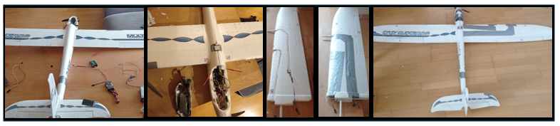
Airframe Instrumentation


Comments