


Hardware components | ||||||
_ztBMuBhMHo.jpg?auto=compress%2Cformat&w=48&h=48&fit=fill&bg=ffffff) |
| × | 1 | |||
| × | 1 | ||||
| × | 1 | ||||
| × | 1 | ||||
| × | 1 | ||||
Gas sensing
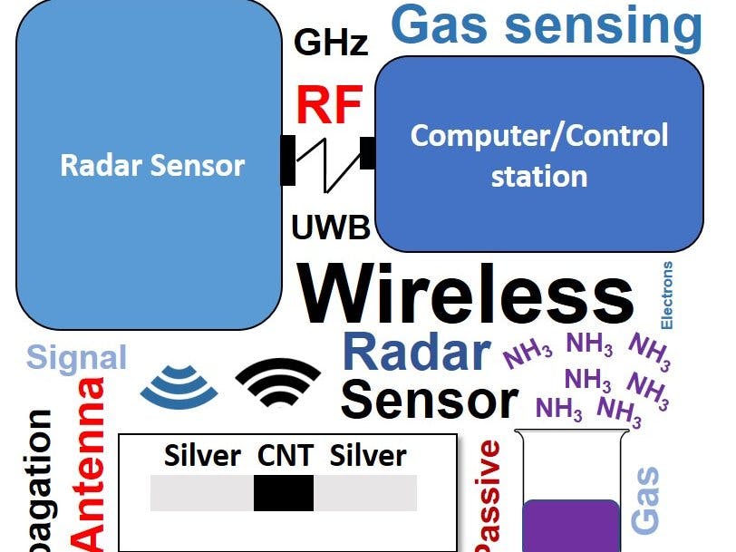
We designed a working prototype for a compact, wireless ammonia gas sensor for real-time gas detection accurate to the ppm range. We coupled a piece of gas sensing film composed of photopaper, carbon nanotubes, and printed silver, with the Walabot Pro.
This project was realized to meet the demands of industries and households for cheap and accessible real-time gas monitoring. There has been an increasing prevalence of volatile compounds found in industrial environments and in common household products, such as in cleaners, coatings of furniture, and even in certain foods! If presented in high concentrations, these volatile compounds, such as ammonia, sulfur, and chlorine, can be hazardous to human health.
However while the demand for real-time gas monitoring has extended to household environments, the technology for gas sensing is currently not at the level where it is readily accessible for the general public. Current commercially available gas sensors are expensive, bulky, and thus inappropriate for household use. While there are low-cost gas sensors on the market, these sensors lack in accuracy, and usually require technical expertise to properly calibrate.
Therefore, we envisioned a gas sensor design that requires no calibration and is both low-cost and compact without compromising accuracy and response time.
How it works
Carbon nanotubes have electrical conductivity that are very sensitive to the presence of small quantities of gas. Upon exposure to a small amount of gas, such as ammonia, the conductivity of the carbon nanotubes will be reduced significantly. We printed a set of silver lines that are placed in contact with the carbon nanotubes to act as antennas. The antennas convert electric current to radio waves operating in the same frequency as the Walabot. The reduction in the conductivity of the carbon nanotube will change the magnitude of the radio waves emitted by the antenna, which we will interrogate with the Walabot. By performing some post processing on the acquired signals, we sort the magnitude readings into the correct ammonia exposure levels, which we measure using a MQ-135 Ammonia Gas sensor module for the Arduino.
How it is made
We created a gas sensing film using photopaper, carbon nanotubes, and printed silver. We deposited the silver onto the photopaper using a paintbrush to create makeshift planar antenna that will interrogate RF signals. Carbon nanotubes are then printed onto the photopaper ensuring that it is in contact with the antennas.
Demonstration Video
Example Plots
An obvious change in the energy and amplitudes of the signals returned by the gas sensing film can be observed when exposed to different concentrations of ammonia gas. Generally, exposure to higher concentrations of ammonia gas will will result in a lo energy and low amplitude.
Walabot Raw Backscattered Signals
Python# --------------------------------------DATA COLLECTION-------------------------------------------
# | File: RawSignalCollection |
# | Type: .py (python) |
# | Purpose: Collects the amplitude values of the backscattered signals from the gas-sensing |
# | films writes those into a csv file named 'ftraw.csv', shows the collected signals in real- |
# | time and saves each frame of collected data as well, for visual representation. | |
# | NOTE: This program should only be used with the short-range-imaging sensor profile. |
# ------------------------------------------------------------------------------------------------
from __future__ import print_function
from sys import platform
from os import system
import WalabotAPI as wlbt
import matplotlib.pyplot as plt
from drawnow import drawnow
# _______________________________________________________________________________________________________
#| COLOR MATRIX |
#| ______________________________________________________________________________________________________|
# The matrix with 40 different colors; this is to be used later when plotting data from the antenna
# pairs. THe size of this matrix is 40 because that correlates with the total number of available
# antenna pairs.
COLORS = [
"000000", "0000FF", "DC143C", "00FFFF", "008000", "0000FF", "ADD8E6", "F8F8FF", "F0FFF0", "6495ED",
"6A5ACD", "FAF0E6", "00008B", "B0E0E6", "2E8B57", "BDB76B", "FFFAFA", "A0522D", "0000CD", "4169E1",
"E0FFFF", "008000", "9370DB", "191970", "FFF8DC", "AFEEEE", "FFE4C4", "708090", "008B8B", "F0E68C",
"F5DEB3", "008080", "9932CC", "FA8072", "00BFFF", "663399", "8B0000", "4682B4", "DB7093", "778899"]
# _______________________________________________________________________________________________________
#| INITIALIZING/CNNECTING WALABOT |
#| ______________________________________________________________________________________________________|
# Load the python WalabotAPI into the program as 'wlbt' and initialize it
wlbt.Init()
wlbt.SetSettingsFolder()
# Establish a connection between the Walabot and the computer
wlbt.ConnectAny()
# Set up the sensing profile; since the optimal results for gas concentration detection
# with the CNT films are obtained at a small distance, the short-range imaging profile is used.
# Also, since we're detecting stationary sensors, the chosen filter type is None.
wlbt.SetProfile(wlbt.PROF_SHORT_RANGE_IMAGING)
wlbt.SetDynamicImageFilter(wlbt.FILTER_TYPE_NONE)
# _______________________________________________________________________________________________________
#| ARENA SETUP |
#| ______________________________________________________________________________________________________|
# Setting up the arena parameters for Walabot, using functions from WalabotAPI
xmin, xmax, xres = -1.0, 1.0, 0.1
ymin, ymax, yres = -1.0, 1.0, 0.1
zmin, zmax, zres = 3.0, 8.0, 0.1
wlbt.SetArenaX(xmin, xmax, xres)
wlbt.SetArenaY(ymin, ymax, yres)
wlbt.SetArenaZ(zmin, zmax, zres)
# ________________________________________________________________________________________________________
#| GET ANTENNA PAIRS AND START WALABOT |
#| _______________________________________________________________________________________________________|
# Get the list of antenna pairs that are available and store it in an array
pair = wlbt.GetAntennaPairs()
# Start the Walabot device
wlbt.Start()
# ________________________________________________________________________________________________________
#| LIVE-UPDATING GRAPH |
#| _______________________________________________________________________________________________________|
# 'ant' stores the number of antenna pairs to be used for data collection
ant = 40
# This command creates a new csv file "ftraw.csv" if one does not exist in the program directory and in
# the case it already exists, it overwrites it
f = open("ftraw.csv", "w+", 0)
# Initializing a zero-filled array, which is then updated with the collected data. The size of the array
# depends on the number of antenna pairs to be used.
signal_list = [[0]]*ant
# Initializing the figure window for plotting
plt.ion()
fig = plt.figure()
# The custom-made function to plot the data, depending on the number of antenna pairs chosen
def makeFig():
# The for loop goes up to the size of 'ant', which is the number of antenna pairs, so that
# the loop can plot data from every antenna pair used.
# 'timeAxis' is a 1D array contining the time domain values for the obtained raw signals.
# 'signal_list' is a multidimensional array (the number of dimensions is equal to antenna
# pairs being used). Each element of the array refers to the obtained signal values for
# the correspoding antenna pair. For example, if the 'number' is 3, then the backscattered
# amplitudes obtained from the 4th antenna pair will be plotted.
# 'COLORS' is used to change the line color for each antenna pair.
for number in range(ant):
plt.plot(timeAxis, signal_list[number], '#'+COLORS[number], linewidth=1.0)
# Using a 'try-and-except' here to allow user to stop the data collection whenever they want
# by using Ctrl+C
try:
j=1 # Counter variable for keeping track of the frame numbers
# The infinite loop that runs until the user stops the program with keyboard interrupt.
# This loop allows the Wlaabot to continuously scan the the arena that has been set.
while True:
# Walabot API function used to initiate the scan
wlbt.Trigger()
# The elements in the previously declared 'signal_list' are cleared. This is done so that
# every time this loop runs, the 'signal_list' is updated with the new values and doesn't
# carry on the previous values. Having the previous values in the list would disrupt the
# plotting because the size of the 'signal_list' wouldn't match the 'timeAxis' in that case.
del signal_list[0:ant]
# The for loop goes up to the number of antenna pairs used. This loop allows the Walabot
# to get the raw signals from each one of the selected number of antenna pairs, for every
# scan.
# 'GetSignal' from WalabotAPI which returns the time domain values and the returned signal
# amplitudes. The data from this function is stored in 'targets' (2D array). The first array
# within 'targets' has the returned signal amplitudes and thus, those values are appended to
# 'signal_list'. The second array in 'targets' contains the time domain values and thus, is
# assigned to the 'timeAxis'
for num in range(ant):
targets = wlbt.GetSignal((pair[num]))
signal_list.append(targets[0])
timeAxis = targets[1]
# Loop for writing the collected data to a csv file.
for i in range(len(signal_list[0])):
for k in range(ant):
f.write(str(signal_list[k][i])+',')
f.write('\n')
# The builtin function which updates the figure, with the plots from the previously defined
# function
drawnow(makeFig)
# To keep track of which frame number it is, the user can choose to either save the image
# for each frame or simply print the frame number, which is represented by 'j' here:
# Saves the graphs from each frame (optional).
plt.savefig("frame"+str(j)+".png")
# print(j)
j+=1
except KeyboardInterrupt:
pass
wlbt.Stop() # stops Walabot when finished scanning
wlbt.Disconnect() # stops communication with Walabot
Data Processing: Signal Energy
MATLAB/*---------------------------------DATA PROCESSING------------------------------------------
| File: DataProcessing |
| Type: .m (matlab) |
| Purpose: Reads the signal files (csv) of different gas concentrations and plots the |
| energy of the returned signals. |
-------------------------------------------------------------------------------------------*/
/* _____________________________________________________________________________________
| DATA PROCESSING DESCRIPTION |
| _______________________________________________________________________________________|*/
/*The purpose of this MATLAB script is to produce a a bar graph that compares the energy
of the returned signals, for different gas concentrations.
Overview of data processing steps:
1) Specific frames from raw data files ('ftraw[num].csv') are read. The background frame
is subtracted from the frame containing signals from the sensor. This data is written
into seperate csv files. For example, '1.csv' would contain the data without background
signals, for the highest gas concentraion.
2) The newly-written '[num].csv' files are read into MATLAB and each signal's amplitude
values are squared and then integrated; these values represent the energy of the signal.
3) The next step is to compare the signal energy values of each antenna pair, for all gas
concentrations; for example, if there were 3 concentrations of gas and two
antenna pairs were used, then we would compare the signal energy at all three
concentrations for antenna pair #1 and then for antenna pair #2, seperately. The
purpose of this comparison is to determine which antenna pair's data follows the
expected trend. The expected trend is that the signal energies should decrease with
increasing ammonia concentration.
4) After finding the antenna pair which follows the previously described trend, the
signal energies from that antenna pair are plotted in a bar graph, for all gas
concentrations.
*/
/* _____________________________________________________________________________________
| FUNCTIONS |
| _______________________________________________________________________________________|*/
// Built-in trapz() function: used in the main program
/* Computes the integral of the input arguments. In the case that the
input argument is a matrix (input arguments in this progrmam are matrices too), trapz()
computes the integral of each colunmn of the matrix.
Input: one argument, which is a matrix in this program
Returns: a row vector containing the integral of each column (length of row vector
in this program dependant on the number of antenna pairs used)
*/
// _____________________________________________________________________________________
// Built-in issorted() function: used in the main program
/* Determines if an array is sorted, i.e. the elements of the array are listed in
ascending order.
Input: one argument, which is a row vector in this program
Returns: a logical scalar; returns 1 if the row vector is sorted, 0 if it is not*/
// _____________________________________________________________________________________
/* _____________________________________________________________________________________
| MAIN PROGRAM |
| _______________________________________________________________________________________|*/
// Choose the 'long' format to show a more accurate representation of the signal values
clc
clear
format long
/*Prompts the user to enter the number of gas concnetrations measured and the number
of antenna pairs used for the measurements.*/
num_of_conc = input('Please enter the number of measured gas concentrations: ');
ant_pairs = input('Please enter the number of antenna pairs used: ');
fprintf(1, '\n');
// Global variables
/* Initializing zero-filled matrices so the program doesn't slow down later*/
Integration_values = zeros(num_of_conc, ant_pairs);
x_use = zeros(8192,40);
antenna_pair = 0;
int_x = zeros(1,num_of_conc);
// 'for' loop for subtracting the background signals and writing that data into a
// new csv file
/* The user is asked to enter the frame number for the sensor's reflected amplitudes
and the frame number for the background signals. The code then reads the data
from 'ftraw[number].csv' files and extracts these specific frames for background
subtraction.
*/
for i = 1:num_of_conc
frame_gas_sensing = input(['Please enter the frame number with recorded signals from the gas sensing film, for concentration ', num2str(i), ': ']);
frame_bg = input(['Please enter the frame with recorded background noise, for concentration ', num2str(i), ': ']);
row_start = (2048*(frame_gas_sensing-1));
row_end = row_start + 2047;
row_start_bg = (2048*(frame_bg-1));
row_end_bg = row_start_bg + 2047;
ftraw_data_gas_sensing = csvread(['ftraw', num2str(i),'.csv'], row_start, 0, [row_start 0 row_end ant_pairs-1]);
ftraw_data_bg = csvread(['ftraw', num2str(i),'.csv'], row_start_bg, 0, [row_start_bg 0 row_end_bg ant_pairs-1]);
subtracted_bg = ftraw_data_gas_sensing - ftraw_data_bg;
csvwrite([num2str(i), '.csv'], subtracted_bg)
disp(sprintf(['Background noise has been subtracted and the data is stored in file ', num2str(i), '.csv\n']))
end
// Nested 'for' loops for calculating signal energy for each antenna pair
/* The outer loop goes up to the number of gas concentrations used, to read
data from sequential csv files. The inner loop goes up to the number of antenna pairs
used. Both these loops are used to index into the Integration_values matrix, which
represent a signal's energy. The signal energies are stored in the Integration_values
matrix of size = num_of_conc by ant_pairs matrix, where each row represents the energy
from different antenna pairs at a certain gas concentration.
*/
for k = 1:num_of_conc
for i = 1:ant_pairs
filename = [num2str(k) '.csv'];
x_use = csvread(filename); // file data read into 'x_use' variable
integral_vector = trapz((x_use.^2)); /* Integral of the squared amplitude values
are calculated using built-in function */
Integration_values(k,i) = integral_vector(i); /* The calculated integrals are stored in
the Integration_values matrix*/
end
end
// 'for' loop to find which antenna pair is the first one to follow the expected
// trend
/* A 'for loop is used to iterate through all columns of the Integration_values matrix. Recall that
each column of this matrix contains signal evergies of different gas concnetrations, and
these values are obtained using the same antenna pair. If the values of a certain column
in Integration_values matrix follows the expected trend (i.e. the values increase as we move down
the column), then the program is instructed to break out of the loop.
*/
bf = false; // flag variable for breaking out of the loop once the antenna pair is determined
for m = 1:ant_pairs
antenna_pair = m; // 'm' represents the antenna pair
col = Integration_values(1:num_of_conc, m); /*'col' contains the data from an individual
column of the Integration_values matrix */
e = issorted(col); /* Built-in function 'issorted' used to check if values
in 'col' are increasing in an acsending order. Function
returns 0 when false and 1, when true. */
if e == 1 /* Condition that verifies if a certain column from Integration_values
has values that are increasing */
bf = true; /* If condition holds, then flag variable is set to true and
the program exits the 'if' block and then 'for loop */
break
elseif e == 0 && antenna_pair == 40 /* In case none of the data from any antenna pair
matches the expected trend */
disp('NOTE: Data does not follow expected trend')
end
if bf,break,end
end
// Plotting the bar graphs of signal energies, at different ammonia concentrations
/* The for loop goes up to the number of concnetrations, to read the signal energies from the
previously determined antenna pair, which follows the trend. In the case that the expected trend
is not followed by any antenna pair, the script plots the data from the last antenna pair.
*/
for f = 1:num_of_conc
int_x(f) = Integration_values(f,antenna_pair);
end
bar(int_x, 0.4,'FaceColor',[0 .5 .5],'EdgeColor',[0 .9 .9],'LineWidth',1.5)
title('Signal Energy of Different Ammonia Conentrations');
xlabel('Concentration');
ylabel('Signal Energy');
Signal_energyREADME.txt
TypescriptINSTRUCTIONS FOR DATA COLLECTION AND DATA PROCESSING
DATA COLLECTION USING WALABOT:
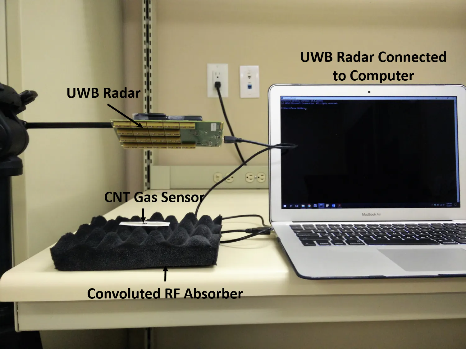
1) Place the gas sensing film under the Walabot (as shown in the video), and start
running the python script, "RawSignalCollection.py" A window with a live-
updating graph will appear, showing the raw signals in real-time. The python
script also provides the option to orint the frame number or save the graph as
'frame[num].png' files, where 'num' represents the frame number.
2) After a few a seonds, remove the gas sensing film from under the Walabot to record
background.
3) Stop the script once you have recorded the background. The raw data will be saved in
'ftraw.csv'.
3) Take note of the specific frame number which contains the signals from the gas sensing film,
and the background data. You will need these two numbers later for data processing.
4) Repeat with different gas concentrations. Make sure to save the 'ftraw.csv' file and
the frame images in another location, or else they will be replaced with the new data
collection.
DATA PROCESSING:
The purpose of this MATLAB script is to produce a a bar graph that compares the energy
of the returned signals, for different gas concentrations.
Here are some things to keep in mind before using this script:
1) All the raw data files obtained through 'RawSignalCollection.py' should be renamed
as 'ftraw[num].csv', where 'num' are integers (1,2,3,..). The file corresponding to
highest gas concentration should be named 'ftraw1.csv', the second highest
concentration should be 'ftraw2.csv' and so on. This naming convention is necessary
for MATLAB script to run properly.
2) These raw data files must be in MATLAB's workspace directory.
3) Enter the number of gas concentrations measured, the number of antenna pairs used,
and the frame numbers for gas sensing film's signals and the background signals,
when prompted.
Data Processing: Fourier Transform
MATLAB/*---------------------------------DATA PROCESSING------------------------------------------
| File: AmmoniaDataProcessing |
| Type: .m (matlab) |
| Purpose: Reads the raw data files (csv) of different gas concentrations and gives |
| a plot of the Fourier Transform of the signals, showing change in amplitude values |
| at various gas concentrations. |
-------------------------------------------------------------------------------------------*/
/* _____________________________________________________________________________________
| DATA PROCESSING DESCRIPTION |
| _______________________________________________________________________________________|*/
/*The purpose of this MATLAB script is to produce a Fourier Transform (FT) graph for each
gas concentration. FT graphs show the frequency composition and amplitudes of signals.
By plotting the FT graphs, we can clearly see the change in signals due to different
gas concentrations.
Overview of data processing steps:
1) Specific frames from raw data files ('ftraw[num].csv') are read. The background frame
is subtracted from the frame containing signals from the sensor. This data is written
into seperate csv files. For example, '1.csv' would contain the data without background
signals, for the highest gas concentraion.
2) The newly-written '[num].csv' files are read into MATLAB and each signal's root-mean-
square (RMS) values are computed. RMS values can be viewed as a signal's strength. Thus,
we obtain the signal strength of each signal, at all the measured gas concentrations.
2) The next step is to compare the RMS values of each antenna pair, for all gas
concentrations; for example, if there were 3 concentrations of gas and two
antenna pairs that were used, then we would compare the RMS values at all three
concentrations for antenna pair #1 and then for antenna pair #2, seperately. The
purpose of this comparison is to determine which antenna pair's data follows the
expected trend. The expected trend is that the RMS values should decrease with
increasing ammonia concentrations.
3) After finding the antenna pair which follows the previously described trend, a FFT
is performed on the signal recorded from that antenna pair, at all concentrations.
The FFT graphs for all concentrations are then plotted in the same figure.
*/
/* _____________________________________________________________________________________
| FUNCTIONS |
| _______________________________________________________________________________________|*/
// Built-in rms() function: used in the main program
/* Computes the root-mean-square (RMS) values of the input arguments. In the case that the
input argument is a matrix (input arguments in this progrmam are matrices too), rms()
computes the RMS values along each colunmn of the matrix.
Input: one argument, which is a matrix in this program
Returns: a row vector containing the rms value of each column (length of row vector
in this program dependant on the number of antenna pairs used)
*/
// _____________________________________________________________________________________
// Built-in issorted() function: used in the main program
/* Determines if an array is sorted, i.e. the elements of the array are listed in
ascending order.
Input: one argument, which is a row vector in this program
Returns: a logical scalar; returns 1 if the row vector is sorted, 0 if it is not*/
// _____________________________________________________________________________________
// Built-in fft() function: used in the custom 'positiveFFT()' function
/* Calculates the FFT of the input argument.
Input: one argument, which is 1D array in this program
Returns: a row vector with the FFT of each indivudal data point, e.g. if the length
of the input array was 2048, the returned row vector will have the same length.
*/
// _____________________________________________________________________________________
// Custom positiveFFT() function: used in the main program
/* Provides the normalized amplitude values for the fft and gets rid of the mirrored
image resulting form the symmtery by only using the first half of the dataset. It
also gives an x-axis that is in terms of frequency (GHz); it uses the dataset and
the sampling rate to determine those frequencies.
Input: two arguments; one is the dataset (1D array) and the the other is a sampling
rate (integer)
Returns: two row vectors
- first vector conatins the normalized FFT amplitude values
- second vector contains the x-axis frequency values
*/
function [ X,freq ] = positiveFFT( x, Fs )
N = length(x); // Taking the length of the input dataset to find the number of samples
k = 0:N-1;
T = N/Fs; // Period
freq = k/T; // Creates the frequency range
X = fft(x)/N; // Normalizes the FFT
upperbound = ceil(N/2);
X = X(1:upperbound); /* Stores only the first half of the dataset values from the fft
to eliminate the mirrored image of the peaks */
freq = freq(1:upperbound); /* Stored the x-axis values corresponding to the first half
of the dataset. */
end
/* _____________________________________________________________________________________
| MAIN PROGRAM |
| _______________________________________________________________________________________|*/
// Choose the 'long' format to show a more accurate representation of the signal values
clc
clear
format long
/*Prompts the user to enter the number of gas concnetrations measured and the number
of antenna pairs used for the measurements.*/
num_of_conc = input('Please enter the number of measured gas concentrations: ');
ant_pairs = input('Please enter the number of antenna pairs used: ');
fprintf(1, '\n');
// Global variables
/* Initializing zero-filled matrices so the program doesn't slow down later*/
RMS_values = zeros(num_of_conc, ant_pairs);
x_use = zeros(2048,40);
antenna_pair = 0;
// 'for' loop for subtracting the background signals and writing that data into a
// new csv file
/* The user is asked to enter the frame number for the sensor's reflected amplitudes
and the frame number for the background signals. The code then reads the data
from 'ftraw[number].csv' files and extracts these specific frames for background
subtraction.
*/
for i = 1:num_of_conc
frame_cnt = input(['Please enter the frame number containing signals from the gas-sensing film for concentration ', num2str(i), ': ']);
frame_bg = input('Please enter the frame with recorded background signals: ');
row_start = (2048*(frame_cnt-1));
row_end = row_start + 2047;
row_start_bg = (2048*(frame_bg-1));
row_end_bg = row_start_bg + 2047;
ftraw_data_cnt = csvread(['ftraw', num2str(i),'.csv'], row_start, 0, [row_start 0 row_end ant_pairs-1]);
ftraw_data_bg = csvread(['ftraw', num2str(i),'.csv'], row_start_bg, 0, [row_start_bg 0 row_end_bg ant_pairs-1]);
subtracted_bg = ftraw_data_cnt - ftraw_data_bg;
csvwrite([num2str(i), '.csv'], subtracted_bg)
disp(sprintf(['Background signals have been subtracted and the data is stored in file ', num2str(i), '.csv\n']))
end
// Nested 'for' loops for calculating the root-mean-square (RMS) values for signals from
// each antenna pair
/* The outer loop goes up to the number of gas concentrations used, to read
data from sequential csv files. The inner loop goes up to the number of antenna pairs
used. Both these loops are used to index into thr RMS-values matrix. The RMS values
are stored in the RMS_values matrix of size = num_of_conc by ant_pairs matrix, where
each row represents the RMS values from different antenna pairs at a certain gas
concentration.
*/
for k = 1:num_of_conc
for i = 1:ant_pairs
filename = [num2str(k) '.csv'];
x_use = csvread(filename); // file data read into 'x_use' variable
RMS_rowvector = rms(x_use); /* RMS values of each cocnentration (i.e. each file)
are calculated using built-in function */
RMS_values(k,i) = RMS_rowvector(i); /* The calculated RMS values are stored in
the RMS_values matrix*/
end
end
// 'for' loop to find which antenna pair is the first one to follow the expected
// trend
/* A 'for loop is used to iterate through all column of the RMS_values matrix. Recall that
each column of this matrix contains RMS values at different gas concnetrations, and
these values are obtained using the same antenna pair. If the values of a certain column
in RMS_values matrix follows the expected trend (i.e. the values increase as we move down
the column), then the program is instructed to break out of the loop.
*/
bf = false; // flag variable for breaking out of the loop once the antenna pair is determined
for m = 1:ant_pairs
antenna_pair = m; // 'm' represents the antenna pair
col = RMS_values(1:num_of_conc, m); /*'col' contains the data from an individual
column of the RMS_values */
e = issorted(col); /* Built-in function 'issorted' used to check if values
in 'col' are increasing in an acsending order. Function
returns 0 when false and 1, when true. */
if e == 1 /* Condition that verifies if a certain column from RMS_values
has values that are increasing */
bf = true; /* If condition holds, then flag variable is set to true and
the program exits the 'if' block and then 'for loop */
break
elseif e == 0 && antenna_pair == 40 /* In case none of the data from any antenna pair
matches the expected trend */
disp('NOTE: Data does not follow expected trend')
end
if bf,break,end
end
// for loop to read through the sequential signal files, specifically the column of the file
// that corresponds to the antenna pair that follows the trend
/* The for loop goes up to the number of concnetrations, to read the sequntial csv files and
extract the column data (stored in fft_x) for the antenna pair determined previously. In the
case that the expected trend is not followed by any antenna pair, the script plots the data
from the last antenna pair.
After the column data is retrieved from the file, it is passed on to 'positiveFFT' function,
which returns the values for the x- and y-values of the FFT graphs. Using this data, the
graphs of FFT for different concnetrations are plotted in the same figure.
*/
Fs = 1e11;
N = 2048;
for f = 1:num_of_conc
// reading data of single antenna pair and computing its fft
fft_x = csvread([num2str(f),'.csv'], 0, antenna_pair-1, [0 antenna_pair-1 N-1 antenna_pair-1]);
[YfreqD,freqRng] = positiveFFT(fft_x,Fs);
// plotting the fft values, along with frequencies in the x-axis
hold on
xlim([3,10])
plot(freqRng/(1e9),abs(YfreqD), 'DisplayName', ['Concentration ',num2str(f)]);
title('FFT Graph of Different Gas Concentrations');
xlabel('Frequency (GHz)');
ylabel('Amplitude (a.u)');
end
legend(gca,'show') // Dynamically updating legend
Fourier_README.txt
TypescriptINSTRUCTIONS FOR DATA COLLECTION AND DATA PROCESSING
DATA COLLECTION USING WALABOT:
1) Place the gas sensing film under the Walabot at 5cm (as shown in the video), and start
running the python script, "RawSignalCollection.py" A window with a live-
updating graph will appear, showing the raw signals in real-time. The python
script also saves the graph of each frame as 'frame[num].png' files, where 'num'
represents the frame number. Alternatively, the user can choose to simply print
the frame number, rather than saving each frame (see python script for more details).
2) After a few a seonds, remove the gas sensing film from under the Walabot to record
background.
3) Stop the script once you have recorded the background. The raw data from this test run
will be saved in 'ftraw.csv'.
4) Take note of the specific frame number which contains the signals from the gas sensing film,
and the background data. You will need these two numbers later for data processing.
5) Repeat with different gas concentrations. Make sure to save the 'ftraw.csv' file and
the frame images in another location, or else they will be re-written when the python script
is used again.
DATA PROCESSING:
The purpose of the MATLAB script is to produce a Fourier Transform (FT) graph for each
gas concentration. FT graphs show the frequency composition and amplitudes of signals.
By plotting the FT graphs, we can clearly see the change in signals due to different
gas concentrations.
Here are some things to keep in mind before using this script:
1) All the raw data files obtained through 'RawSignalCollection.py' should be renamed
as 'ftraw[num].csv', where 'num' are integers (1,2,3,..). The file corresponding to
highest gas concentration should be named 'ftraw1.csv', the second highest
concentration should be 'ftraw2.csv' and so on. This naming convention is necessary
for the MATLAB script to run properly.
2) The raw data files must be saved in MATLAB's workspace directory.
3) Enter the number of gas concentrations measured, the number of antenna pairs used,
and the frame numbers for the gas sensing film's signals and the background signals,
when prompted.


Comments