Published December 15, 2016 © CC BY-NC-SA

RBB Part 2 Motor Position Control

The next part for this project is making the DC motor move to a desired position.

AdvancedFull instructions provided5 hours1,321

Things used in this project

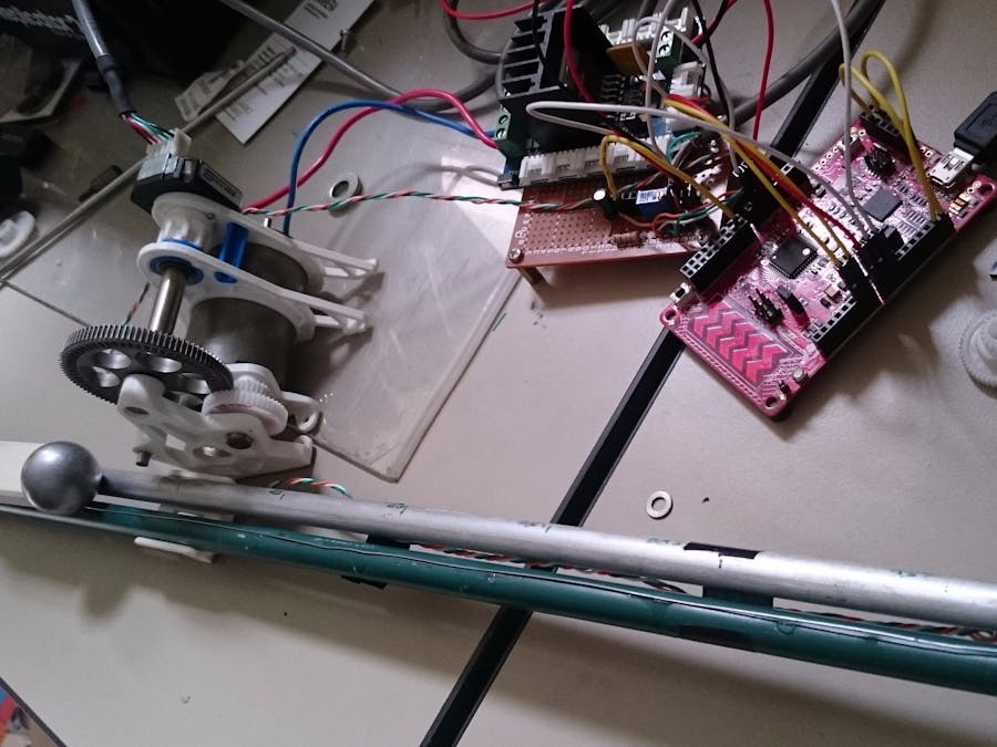
Hardware components

Cypress PSoC 4 Pioneer Kit

DC motor (generic)

SparkFun Dual H-Bridge motor drivers L298

Texas Instruments Dual H-Bridge motor drivers L293D

SparkFun RedBot Sensor - Wheel Encoder

Software apps and online services

Cypress PSoC Creator

MATLAB

Story

Introduction

Continuing the Ball and Beam Part 1 project now we require to control the Motor output angle this will be done with the use of a recursive 2DOF PID controller.

Matlab simulink DC motor control model

The controller

I will not go into detail on how to get the recursive algorithm it involves a lot of math and equation solving. What you need to know about the controller is how it works:

R - Reference Signal (Setpoint/Desired output)

Beta - Proportional reference weight (Range 0-1)

Gamma - Derivative reference weight (Range 0-1)

I - Integral Control (Cumulative error)

P - Proportional Control (Error Magnitude)

D - Derivative Control (Slope of the error or error rate of change )

U - Controller output/Control signal

D - Disturbance (external influences that cannot be measured)

Gp - Plant (the actual system to be controlled, in this case is the motor and gearbox)

Y - Output

Since the algorithm is in recursive form we only need to store the last three values of each reference signal, control signal, and output:

Controller recursive equation

Now to the code.

First we initialize the required variables the whole first line will be used for the equation constants calculations, the second line has all the variables that will be constantly updated.

double aA,aB,aC,aD,aE,aF,aG,aH,aI,aJ,aTd,apP,apI,apD,aWD,aWK,apN,aTf; 
float uX,uXold1,uXold2,uXold3,rX,rXold1,rXold2,rXold3,X,Xold1,Xold2,Xold3,SPX;

Now the initialization of the PID algorithm the first line contains all the modifiable parameters apP , apI, apD , apN , aWK , aWD , aTf .

apP=7;apI=125;apD=0;apN=2000;aWK=0.6;aWD=0,aTf=0.00003;   
initpidang();                
SPX=1; 
uX=0; uXold1=0;uXold2=0;uXold3=0; 
X=0;   Xold1=0; Xold2=0; Xold3=0; 
rX=0; rXold1=0;rXold2=0;rXold3=0;

In order to give the processor less tasks or math operations I simplified the equation and separated each coefficient, so after initializing the variables the full equation only uses constant coefficients.

void initpidang (void){        //2dofPID      
   aA=1/(apN*Ts); 
   aB=aA*(apN*Ts-1); 
   aC=aA*(apP*apN*Ts*aWK+apI*Ts*Ts*apN); 
   aD=aA*(aWK*apP-aWK*apP*apN*Ts+apI*Ts+apD*apN*aWD); 
   aE=aA*(-2*apP*aWK-apI*Ts-2*apD*apN*aWD); 
   aF=aA*(apP*aWK+apD*apN*aWD); 
   aG=aA*(-apP*apN*Ts-apI*Ts*Ts*apN); 
   aH=aA*(-apP+apP*apN*Ts-apI*Ts-apD*apN); 
   aI=aA*(2*apP+apI*Ts+2*apD*apN);    
   aJ=aA*(-apP-apD*apN); 
}

And finally the actual control loop first line is the controller equation. Second and third lines limit the maximum and minimum output. Fourth line is just motor command update and the last ones are the values updating to the current set.

uX=uXold1*aB-2*uXold2*aA-uXold3*aA+aC*rX+aD*rXold1+aE*rXold2+aF*rXold3+aG*X+aH*Xold1
    +aI*Xold2+aJ*Xold3;
if(fabs(uX)>(PWMmaxper-1)){mot=(PWMmaxper-1)*fabs(uX)/uX;}
else{mot=uX;} 
motoroutput();
uXold3=uXold2; uXold2=uYold1; uXold1=motspd; 
Xold3=Xold2; Xold2=Xold1; Xold1=X; X=ang;
rXold3=rXold2; rXold2=rXold1; rXold1=rX; rX=SPX;

Here is an example of how using the current ball position value the motor gets an equivalent angle reference and follows it.

Using Micruim uProbe the variables can be plotted easily notice the green line Set point is exactly the ball position divided by 10.

notice also the curve shape is very similar between them

Code

Program Code

* ========================================
 * Copyright Juan Esteban Paz, 2014
 * All Rights Reserved
 * UNPUBLISHED, LICENSED SOFTWARE.
 * ========================================*/
//$ STOP //# PRBS //& OpenLoop  //" POS  //% Angle //* Print on off

#include <project.h>
#include <ballbeam.h>
#include <math.h>
//function prototypes
void Init();
CY_ISR(UARTRX);
//constants
int tcomp,t,c,a=1,angle,e=0,run=0,print=0,i=0,location,adcCounts;
double ang,counter,Xpos,meas,Ts=0.0015;
int motspd=0;

double aA,aB,aC,aD,aE,aF,aG,aH,aI,aJ,aTd,apP,apI,apD,aWD,aWK,apN,aTf;        
float uX,uXold1,uXold2,uXold3,rX,rXold1,rXold2,rXold3,X,Xold1,Xold2,Xold3, SPX;


void initpidang (void){        //2dofPID     
    aA=1/(apN*Ts);
    aB=aA*(apN*Ts-1);
    aC=aA*(apP*apN*Ts*aWK+apI*Ts*Ts*apN);
    aD=aA*(aWK*apP-aWK*apP*apN*Ts+apI*Ts+apD*apN*aWD);
    aE=aA*(-2*apP*aWK-apI*Ts-2*apD*apN*aWD);
    aF=aA*(apP*aWK+apD*apN*aWD);
    aG=aA*(-apP*apN*Ts-apI*Ts*Ts*apN);
    aH=aA*(-apP+apP*apN*Ts-apI*Ts-apD*apN);
    aI=aA*(2*apP+apI*Ts+2*apD*apN);   
    aJ=aA*(-apP-apD*apN);
}
void initpidpos (void){                
bb=1/(bpN*Ts);
bB=bb*(bpN*Ts-1);
bC=bb*(bpP*bpN*Ts*bWK+bpI*Ts*Ts*bpN);
bD=bb*(bWK*bpP-bWK*bpP*bpN*Ts+bpI*Ts+bpD*bpN*bWD);
bE=bb*(-2*bpP*bWK-bpI*Ts-2*bpD*bpN*bWD);
bF=bb*(bpP*bWK+bpD*bpN*bWD);
bG=bb*(-bpP*bpN*Ts-bpI*Ts*Ts*bpN);
bH=bb*(-bpP+bpP*bpN*Ts-bpI*Ts-bpD*bpN);
bI=bb*(2*bpP+bpI*Ts+2*bpD*bpN);   
bJ=bb*(-bpP-bpD*bpN);  
}

CY_ISR(ADCEOC){   
    //y = -0.6423x + 404.66*R² = 0.9944
    //ADC_StopConvert();    
    adcCounts = ADC_GetResult16(CH0);
    meas= ADC_CountsTo_uVolts(CH0,adcCounts);   
    //x=meas;    
    Xpos=-0.6423*meas/1000+322.6;//+comp 
   // ADC_StartConvert();     
}
void motoroutput(){
    if((motspd>=0)&&(motspd<Motcontscale)){
        PWMSpd_WriteCompare(motspd); 
        CCW();       
	}
	else if ((motspd<0)&&(motspd>-Motcontscale)){        
		PWMSpd_WriteCompare(-motspd); 
        CW();
	}	    
}
void message(){
	NewLine();	
    itoa(ang*100,msg,10);//int,char,int base (2,8,10)		
	UART_UartPutString(msg);//ang
	itoa(motspd,msg,10);
	UART_UartPutString(" ");//power	
	UART_UartPutString(msg);
    //itoa(x*10,msg,10);
	UART_UartPutString(" ");//x	
	//UART_UartPutString(msg);
    t=TimerA_ReadCounter();
    itoa(t,msg,10);    
	UART_UartPutString(" ");//time	
	UART_UartPutString(msg);
	UART_UartPutString("f");    
}
void Uartdec(char ch){
 //UART DECODING					
    switch(ch){                            
    	case('1'):{	////STOP///		   											
    		motspd=0;
    		motoroutput(); 	
            e=1;
    		NewLine();
            PWMSpd_Stop();
            ControlReg_Write(0u);  	
    		NewLine();
    		TimerA_Stop();
            UART_UartPutString("Stopped");	
    		run=0;
    		print=0;
            
    		break;}	////STOP///	
        case('2'):{//position control
            
            apP=7;apI=125;apD=0;apN=2000;aWK=0.6;aWD=0,aTf=0.00003;  
            initpidang();               
            SPX=1;
            uX=0; uXold1=0;uXold2=0;uXold3=0;
            X=0;   Xold1=0; Xold2=0; Xold3=0;
            rX=0; rXold1=0;rXold2=0;rXold3=0;     
            ADC_StartConvert();
            ISRADCEOC_Enable();
            UART_UartPutString("Control Mode ANG");
       		e=5;						
    		TimerA_WriteCounter(0);TimerA_Start();
            motspd=0;motoroutput();PWMSpd_Start(); 	
    		run=1;  
            NewLine();
    		break;}//ModoControl ANG 2DOF PID 
    }	
}

int main()
{       
    CyGlobalIntEnable;
    Init();	
    int i=0;
	for(;;){
        //Encoder Reading -> angle///
        counter=QuadDec_GetCounter();
        ang=counter/encres/4*2*PI;//beamdeg
        //Running Modes
		switch(e){		
			
            case(2):{
                
                SPX=Xpos/50;
                uX=uXold1*aB-2*uXold2*aA-uXold3*aA+aC*rX+aD*rXold1+aE*rXold2+aF*rXold3+aG*X+aH*Xold1+aI*Xold2+aJ*Xold3;
                uX=aTf*(uX-uXold1)/Ts+uXold1;            	
                    
                motspd=uX*100;
                motoroutput();
                uXold3=uXold2; uXold2=uYold1; uXold1=uX;                
                Xold3=Xold2; Xold2=Xold1; Xold1=X; X=ang;
                rXold3=rXold2; rXold2=rXold1; rXold1=rX; rX=SPX;

                itoa((rX-X)*100,msg,10);UART_UartPutString(msg);UART_UartPutString(" ");	            
                itoa(SPX*100,msg,10);UART_UartPutString(msg);UART_UartPutString(" ");               
                t=TimerA_ReadCounter();itoa(t,msg,10);UART_UartPutString(" ");UART_UartPutString(msg);//time	
            	UART_UartPutString("f");
				NewLine();
                break;
            }//ModoControl ANG I-PD Filtered          
		}
	}    
}
void Init(){            
    UART_Start();
	UART_UartPutString("Ball&BeamV2");	
	QuadDec_SetCounter(0);
    QuadDec_Start();       
    ///ADC
    ADC_Start();
    ADC_StartConvert();
    opamp_Start();    
    ISRADCEOC_StartEx(ADCEOC);
    UARTISR_StartEx(UARTRX);
}
CY_ISR(UARTRX){
    UARTISR_Disable();
    ch=UART_UartGetChar(); //UART_UartPutChar(ch);  
	if (0!=ch) Uartdec(ch);       
    UART_ClearRxInterruptSource(UART_INTR_RX_NOT_EMPTY);
    UARTISR_Enable();    
}

Credits

Juan Esteban Paz

13 projects • 27 followers

Mechanical and Electrical Engineer enjoy working with PSOC

RBB Part 2 Motor Position Control

Things used in this project

Hardware components

Software apps and online services

Story

Introduction

The controller

Now to the code.

Schematics

PSoC Project RBB part2

Code

Program Code

Credits

Juan Esteban Paz

Comments

Embed the widget on your own site

RBB Part 2 Motor Position Control

RBB Part 2 Motor Position Control

Things used in this project

Hardware components

Software apps and online services

Story

Introduction

The controller

Now to the code.

Schematics

PSoC Project RBB part2

Code

Program Code

Credits

Juan Esteban Paz

Comments

Related channels and tags