


Hardware components | ||||||
 |
| × | 3 | |||
 |
| × | 1 | |||
| × | 1 | ||||
| × | 1 | ||||
Software apps and online services | ||||||
 |
| |||||
| ||||||
Hand tools and fabrication machines | ||||||
 |
| |||||
 |
| |||||
If you spend your days in Fusion 360, Solidworks, Blender or any other 3D CAD program, you’ve probably wished for a better way to navigate the 3d world than the classic mouse + keyboard combo..
After some research you might have come across something called a 3D Space Mouse and thought: I’m a Maker! Why not try building it on my own? Well you’re not alone!So here is our take on the problem, including a full build guide including assembly, coding, and calibration.We also provide a full build guide: Assembly, coding, and calibration. Ready to dive in?
What is a 3D space mouse?A 3D space mouse is an input device that provides control over six degrees of freedom: translation and rotation along the X, Y and Z axes(2x3 = 6 degrees). Instead of using separate controls for pan, tilt and zoom, a 6‑DoF controller lets you apply all these motions simultaneously. With our device, this can be done by pushing, pulling, tilting and twisting a single knob using only one hand. This is far more natural for manipulating 3D models or camera views and means faster navigation, more intuitive manipulation, and fewer context switches.
How does it detect the Position?We measure the knob’s position and rotation using three 3D magnetic sensors, each paired with a magnet. Each sensor reports a 3D magnetic field vector (in mT), giving us three vectors in total.These readings correspond to the 3D positions of an imaginary triangle’s corners on the knob. From those three points, we compute a single rigid transform (rotation + translation) to recover the knob’s full 6‑DoF pose. For the background knowledge, see this article; for the setup and usage, see this article.
High‑level design choices
- Contactless sensing: Magnetic sensors measure fields without mechanical contact on the moving part. The top piece only uses magnets; no wires, slip rings, or connectors. This reduces failure modes and simplifies assembly.
- Minimal moving parts: The knob floats on three springs and holds three magnets. That keeps the moving assembly light and reliable.
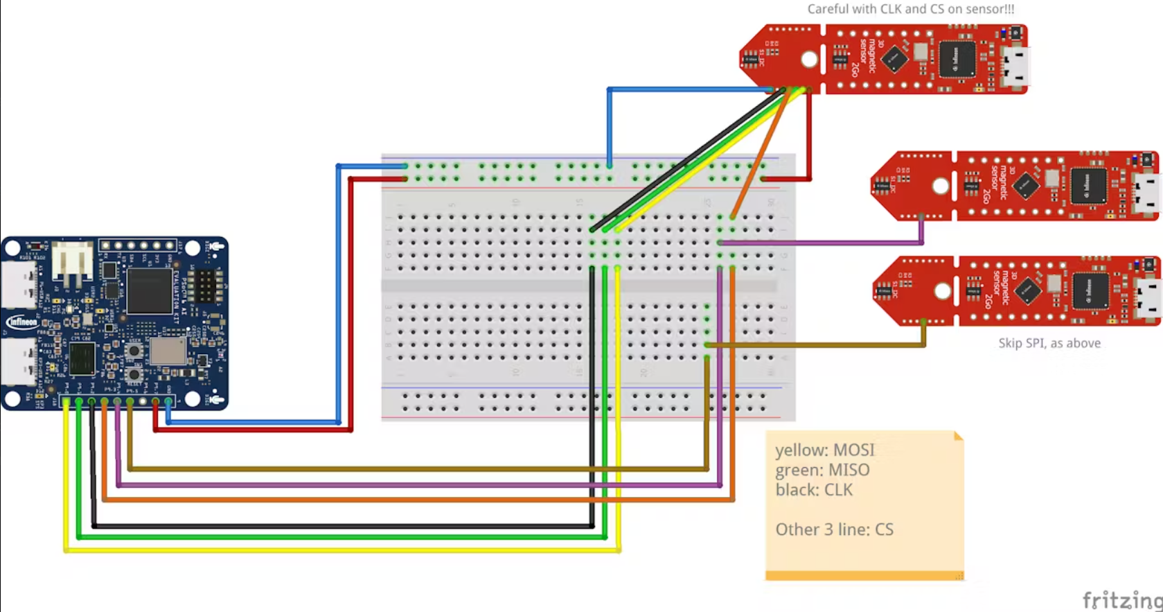
- Simple wiring: We use three sensor breakouts chained to one MCU using a common SPI bus (shared VDD/GND/SCLK/MISO/MOSI) with one chip‑select per sensor. An 8‑wire cable leaves the base (5 common wires + 3 CS).
1) Prepare the printed parts: fit M2.5 heat‑set inserts where screws are needed. We decided to print it out of ABS to achieve a smoother look. To do this, the print needs to be in a vapor chamber filled with aceton. This is entirely optional and comes with a warning: Aceton is toxic when inhaled in high doses and can be irritating to the eyes. Be safe!
2) Mount sensors: screw the three breakout sensors into the triangular sensor base.Solder the VDD, GND, SCLK, MISO, and MOSI lines to all sensors, and assign a dedicated CS to each sensor. Route the 8‑wire cable (VDD, GND, SCLK, MISO, MOSI, CS1, CS2, CS3) out through the base hole, and connect everything as shown in the attached Fritzing diagram.The soldering is relatively difficult because the holes are only 1.27 mm apart.
3) Route cables: pass the cable through the base hole and mount the MCU behind the sensor block. Bild einfügen
4) Add mass: place metal weight plate(s) in the bottom of the base and fasten the cover with screws.
5) Build the knob: place the three magnets in the magnet holder and fasten. Place the three springs into the knob seats and use a bit of hot glue the three springs into the whole (without restricting their movement). Attach the magnet holder to the top of the knob and secure.
6) Final assembly: place the knob assembly over the sensors so the magnets face the sensors at neutral. Verify the knob moves freely and springs return it to center.
Now the Hardware assembly is completed. :)
Calibration and mapping conceptWe map raw sensor readings into a useful coordinate frame in a few steps:
1) Min–Max calibration: move the knob through its workspace while recording per‑sensor per‑axis min and max values. This lets us normalize raw readings into a canonical [-1, +1] range.
2) Neutral capture: hold the knob at rest and average several seconds of normalized readings to compute neutral offsets. This centers the mapping so rest corresponds to zero displacement.
3) Local mapping: normalized, zeroed vectors become local 3D points (in meters) for each of the three top corners. For example we map normalized XY to ±XY_HALF_RANGE (meters around center) and the Z component to REST_HEIGHT ± Z_HALF_RANGE.
4) Pose solve: given the known body geometry of the top triangle (learned at neutral) and the three measured world corner positions, compute the rigid transform (rotation R and translation t) using the Kabsch algorithm (SVD) — this gives the full 6‑DoF pose.
Software Architecture — Data-flow OverviewFirst, the microcontroller (MCU) continuously polls sensor values via SPI and transmits this data to the connected PC through UART.On the PC, a Python script receives and parses the incoming sensor data, than calculates the knob’s rotation and translation values.
Arduino AlgorithmThe following paragraph explains how to read the Data from the sensors with arduino. But we also provide Code for the ModusToolBox if you want to program the PSOC™ 6.
Pin assignment and sensor instances
First include the 3D Magnetic Library for the sensors. Here is a hackster article how you can do that and how to to use the library.
Than you have to define the pins where the sensors are connected and which SPI bus you are using (here the standard SPI bus).
#include "TLx493D_inc.hpp"
using namespace ifx::tlx493d;
/** Definition of the power and chip select pins for 3 sensors. */
/** Sensor 1 */
const uint8_t POWER_PIN_1       = 7;
const uint8_t CHIP_SELECT_PIN_1 = 4;
/** Sensor 2 */
const uint8_t POWER_PIN_2       = 7;
const uint8_t CHIP_SELECT_PIN_2 = 5;
/** Sensor 3 */
const uint8_t POWER_PIN_3       = 7;
const uint8_t CHIP_SELECT_PIN_3 = 6;
/** Declaration of the sensor objects. */
TLx493D_P3I8 sensor1(SPI);
TLx493D_P3I8 sensor2(SPI);
TLx493D_P3I8 sensor3(SPI);Pin assignment and sensor instances.
Setup We start the serial communication at 115200 baud, then configure and initialize all three TLx493D sensors (power pins, chip‑select pins, and SPI). A short delay allows the hardware to stabilize.
void setup() {
Serial.begin(115200);
while (!Serial) ;
/** Initialize Sensor 1 */
sensor1.setPowerPin(POWER_PIN_1, OUTPUT, INPUT, HIGH, LOW, 1000, 250000);
sensor1.setSelectPin(CHIP_SELECT_PIN_1, OUTPUT, INPUT, LOW, HIGH, 0, 0, 0, 5);
sensor1.begin(true, true);
/** Initialize Sensor 2 */
sensor2.setPowerPin(POWER_PIN_2, OUTPUT, INPUT, HIGH, LOW, 1000, 250000);
sensor2.setSelectPin(CHIP_SELECT_PIN_2, OUTPUT, INPUT, LOW, HIGH, 0, 0, 0, 5);
sensor2.begin(true, true);
/** Initialize Sensor 3 */
sensor3.setPowerPin(POWER_PIN_3, OUTPUT, INPUT, HIGH, LOW, 1000, 250000);
sensor3.setSelectPin(CHIP_SELECT_PIN_3, OUTPUT, INPUT, LOW, HIGH, 0, 0, 0, 5);
sensor3.begin(true, true);
delay(200);
}LoopAnd in the loop the magnetic values are measured and printed via Serial communication so that in the end a string with this magnetic values is sent.
void loop() {
double temp = 0.0;
double x1 = 0.0, y1 = 0.0, z1 = 0.0;
double x2 = 0.0, y2 = 0.0, z2 = 0.0;
double x3 = 0.0, y3 = 0.0, z3 = 0.0;
/** Read magnetic field values from all three sensors. */
sensor1.getMagneticFieldAndTemperature(&x1, &y1, &z1, &temp);
sensor2.getMagneticFieldAndTemperature(&x2, &y2, &z2, &temp);
sensor3.getMagneticFieldAndTemperature(&x3, &y3, &z3, &temp);
// Send data in format: x1,y1,z1,x2,y2,z2,x3,y3,z3
// Values are in mT (millitesla)
Serial.print(x1, 2);
Serial.print(",");
Serial.print(y1, 2);
Serial.print(",");
Serial.print(z1, 2);
Serial.print(",");
Serial.print(x2, 2);
Serial.print(",");
Serial.print(y2, 2);
Serial.print(",");
Serial.print(z2, 2);
Serial.print(",");
Serial.print(x3, 2);
Serial.print(",");
Serial.print(y3, 2);
Serial.print(",");
Serial.print(z3, 2); // println adds newline at the end
Serial.println();
}A calibration UI facilitates accurate measurements: it provides two buttons: 1. Calibrate Min-Max (15 s), ” which expects movement across the workspace, and 2. “Capture Neutral (5 s), ” where the knob should remain stationary in the neutral position. The following pictures shows, how you can calibrate the algorithm.Before you start, you have only a triangle (picture 1), after the calibration you have a prism (picture 2) which you can tilt or rotate around the axis (picture 3).
During processing, the system normalizes raw sensor values, subtracts neutral offsets, maps the data to local meter units, constructs world coordinate corner points, and computes rotation and translation (R, t) using the Kabsch algorithm.
The output module converts the pose to the desired format (Euler angles or quaternion plus translation), optionally amplifies translation, and sends it to target applications or a visualization tool.These processed values feed a Fusion add‑in, which interprets them and controls your block within the design environment.
1) Parsing the UART Line
We expect each line to be nine comma separated floats: x1, y1, z1, x2, y2, z2, x3, y3, z3.
def parse_uart_line(line):
Expect 9 comma-separated floats: x1, y1, z1, x2, y2, z2, x3, y3, z3
Each triple is one sensor's raw 3-axis reading.
Returns a list of 9 floats or None on parse failure.
try:
vals = [float(x) for x in line.strip().split(',') if x]
if len(vals) == 9:
return vals
except Exception:
pass
return None
Why this matters: clean parsing is the first step. If your MCU changes format, adjust this function.
2) Min–max Normalization
We map raw axis values from sensor‑specific ranges into a unified [-1, +1] domain.
def minmax_normalize(vec, vmin, vmax):
"""
Normalize vec component-wise into [-1, +1] using per-axis vmin/vmax.
Protects against zero ranges.
"""
vec = np.asarray(vec, dtype=float)
vmin = np.asarray(vmin, dtype=float)
vmax = np.asarray(vmax, dtype=float)
denom = vmax - vmin
out = np.zeros_like(vec)
mask = denom > 1e-12
out[mask] = (vec[mask] - vmin[mask]) / denom[mask]  # [0..1]
out = np.clip(out, 0.0, 1.0)
out = (out * 2.0) - 1.0  # -> [-1..1]
return out
```
Notes: protection against division by zero. After this, each axis is relative to its observed min and max.
3) Map normalized values to local meters
After subtracting the neutral offset (so rest maps to zero), we interpret the normalized vector as a local displacement. Once neutral is subtracted, the normalized vector is interpreted as local displacements (meters) per axis.
def local_from_normalized(n_zero, xy_half_range=0.05, rest_height=0.20, z_half_range=0.05):
"""
Map normalized zero-centered vector n_zero to a local 3D point (meters)
relative to the corresponding base corner.
"""
nx, ny, nz = n_zero
return np.array([
xy_half_range * nx,                    # local x (meters)
xy_half_range * ny,                    # local y (meters)
rest_height + z_half_range * nz        # local z (meters) around rest height
], dtype=float)
Interpretation: choose XY_HALF_RANGE and Z_HALF_RANGE to match mechanical travel and desired sensitivity.
4) Build world corner points
Each sensor has a local frame; we convert the local point into world coordinates:
Qi = base_corner_world[i] + R_local_to_world[i] @ local_m_flipped
- base_corner_world[i] is the fixed world position of the sensor mounting point (the base triangle corner).
- R_local_to_world[i] orients the sensor’s local axes into global axes.
- local_m_flipped is the raw local measurement after applying any needed per-axis sign inversions to account for sensor mounting polarity.
5) Kabsch algorithm — solve for rigid transform
Once we have P_body (the top triangle corners in body coordinates, learned at neutral) and Q_world (measured world corner positions), we find R and t so that R @ P_body + t ≈ Q_world.
```python
def kabsch_rigid_transform(P, Q):
"""
Kabsch: compute rotation R and translation t that maps points P -> Q.
P, Q: (N,3) arrays with matching point order. Returns R (3x3) and t (3,).
"""
P = np.asarray(P, dtype=float)
Q = np.asarray(Q, dtype=float)
assert P.shape == Q.shape and P.shape[1] == 3
p_mean = P.mean(axis=0)
q_mean = Q.mean(axis=0)
Pc = P - p_mean
Qc = Q - q_mean
H = Pc.T @ Qc
U, S, Vt = np.linalg.svd(H)
R = Vt.T @ U.T
# Reflection safeguard
if np.linalg.det(R) < 0:
Vt[2, :] *= -1.0
R = Vt.T @ U.T
t = q_mean - R @ p_mean
return R, t
```
Why Kabsch? For rigid bodies, the Kabsch (SVD) solution gives the optimal rotation and translation that aligns two corresponding point sets. With three non‑colinear points it is exact except for sensor noise.
6) Putting it all together — runtime flow (pseudocode)
- Read a line from UART and parse into nine floats.
- For i in 0..2:
- v_raw = vals[3*i : 3*i+3]
- v_norm = minmax_normalize(v_raw, calib_min[i], calib_max[i])
- n_zero = v_norm - neutral_offsets[i]
- local_m = local_from_normalized(n_zero)
- local_m_flipped = S_local[i] @ local_m
- Qi = base_corner_world[i] + R_local_to_world[i] @ local_m_flipped
- Q_world = stack(Q0,Q1,Q2)
- If P_body known:
- R, t = kabsch_rigid_transform(P_body, Q_world)
- Convert R to Euler angles/quaternion + use t as translation
- Optionally apply translation gain, smoothing, or send to apps- Min‑max capture (15 s): move knob across full workspace to populate per‑axis min and max.
- Neutral position (5 s): rest knob at neutral for neutral_offsets. This also lets us learn P_body corners by computing the neutral Qi values and subtracting the centroid to get body‑frame corner vectors.
- Smoothing: use a small moving average on the last N samples (N ~ 3–8) to reduce jitter.
- Amplification: translation for visualization or control sensitivity can be amplified independently of rotation.
- Axis flips: if a sensor is mounted flipped, apply a per‑sensor sign flip in S_local.
Now we are at the final step. :)
First we need to create a AddIn called MyAddIn and it will locate at "Autodesk Fusion 360\API\AddIns\MyAddIn", then place 3DMouseControllerAddIn.py in file MyAddIn.py.
After that you have to press ADD-IN and then Scripts and Add-INS (like in the following picture).After that a window opens and you have to turn it on.
- That’s it—now you can control your model with your custom-built 3D SpaceMouse.
If something feels off, don’t worry—these quick checks usually fix it. :) - If pose is unstable: check grounding, sensor power decoupling, ensure sensors have sufficient dynamic range (adjust magnet strength or sensor distance), and add smoothing.
- If entire device reads biased: recompute neutral offsets in the target environment — magnetic backgrounds matter.
- If rotation is wrong sign: check sensor orientation and use S_local to flip axes.
- Spring stiffness matters: try different springs until the feel matches what you want; lighter springs make the knob float easily, heavier springs provide stronger centering.
Thank you for reading! We are still working on this product to create a cheaper and more maker-friendly solution for comfortable CAD design.The next step is using this prototype and enabling HID, so that we can connect to the PC like a normal Bluetooth mouse. :) Feel free to look up the project in this GitHub repository, like comment and stay tuned for more!


Comments