


Hardware components | ||||||
 |
| × | 1 | |||
_wzec989qrF.jpg?auto=compress%2Cformat&w=48&h=48&fit=fill&bg=ffffff) |
| × | 1 | |||
Software apps and online services | ||||||
 |
| |||||
Main article: https://paulplusx.wordpress.com/2016/03/04/rtpts_mpu/
Motion Processing is an important concept to know. If you want to interact with real time data you should be able to interact with motion parameters such as: linear acceleration, angular acceleration, and magnetic north.
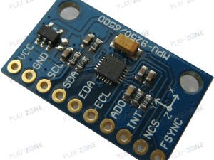
The MPU9250 has an accelerometer, gyroscope, and a magnetometer. The information that we can get from a MPU9250’s are: yaw angle, pitch angle, and roll angle. Given that, I will only deal with yaw here in this post.
The MPU has a 16-bit register for each of its three sensors. They temporarily store the data from the sensor before it is relayed via I2C.
Reading Data
We receive the data 8-bits at a time and then concatenate them together to form 16-bits again. As shown in the following snippet from kriswiners code:
fifo_count = ((uint16_t)data[0] << 8) | data[1];
packet_count = fifo_count/12;// How many sets of full gyro and accelerometer data for averaging
for (ii = 0; ii < packet_count; ii++) {
int16_t accel_temp[3] = {0, 0, 0}, gyro_temp[3] = {0, 0, 0};
readBytes(MPU9250_ADDRESS, FIFO_R_W, 12, &data[0]); // read data for averaging
accel_temp[0] = (int16_t) (((int16_t)data[0] << 8) | data[1]  ) ;  // Form signed 16-bit integer for each sample in FIFO
accel_temp[1] = (int16_t) (((int16_t)data[2] << 8) | data[3]  ) ;
accel_temp[2] = (int16_t) (((int16_t)data[4] << 8) | data[5]  ) ;
gyro_temp[0]  = (int16_t) (((int16_t)data[6] << 8) | data[7]  ) ;
gyro_temp[1]  = (int16_t) (((int16_t)data[8] << 8) | data[9]  ) ;
gyro_temp[2]  = (int16_t) (((int16_t)data[10] << 8) | data[11]) ;
accel_bias[0] += (int32_t) accel_temp[0]; // Sum individual signed 16-bit biases to get accumulated signed 32-bit biases
accel_bias[1] += (int32_t) accel_temp[1];
accel_bias[2] += (int32_t) accel_temp[2];
gyro_bias[0]  += (int32_t) gyro_temp[0];
gyro_bias[1]  += (int32_t) gyro_temp[1];
gyro_bias[2]  += (int32_t) gyro_temp[2];
}
Calibrating the Raw Data
The data that is received then must be calibrated according to the users environment. The calibration of the magnetometer is required to compensate for Magnetic Declination. The exact value of the correction depends on the location. There are two variables that have to calibrated: yaw and magbias.
The below shows yaw calibration for a specific magnetic declination (at Potheri, Chennai, India). The declination data can be obtained from different sites:
yaw   = atan2(2.0f * (q[1] * q[2] + q[0] * q[3]), q[0] * q[0] + q[1] * q[1] – q[2] * q[2] – q[3] * q[3]);
pitch = -asin(2.0f * (q[1] * q[3] – q[0] * q[2]));
roll  = atan2(2.0f * (q[0] * q[1] + q[2] * q[3]), q[0] * q[0] – q[1] * q[1] – q[2] * q[2] + q[3] * q[3]);
pitch *= 180.0f / PI;
yaw   *= 180.0f / PI;
yaw   += 1.34; /* Declination at Potheri, Chennail ,India  Model Used:    IGRF12    Help
Latitude:    12.823640° N
Longitude:    80.043518° E
Date    Declination
2016-04-09    1.34° W  changing by  0.06° E per year     (+ve for west )*/
See the below snippet [the given snippet the data for calibration of magbias comes from another function (magcalMPU9250(float * dest1, float * dest2)):
readMagData(magCount);  // Read the x/y/z adc values
getMres();
//    magbias[0] = +470.;  // User environmental x-axis correction in milliGauss, should be automatically calculated
//    magbias[1] = +120.;  // User environmental x-axis correction in milliGauss
//    magbias[2] = +125.;  // User environmental x-axis correction in milliGauss
// Calculate the magnetometer values in milliGauss
// Include factory calibration per data sheet and user environmental corrections
mx = (float)magCount[0]*mRes*magCalibration[0] – magBias[0];  // get actual magnetometer value, this depends on scale being set
my = (float)magCount[1]*mRes*magCalibration[1] – magBias[1];
mz = (float)magCount[2]*mRes*magCalibration[2] – magBias[2];
}This is one of the simplest and important part of the MPU code. The function magcalMPU9250(float * dest1, float * dest2) calibrates the magnetometer while you move the sensor in a figure eight. It stores the maximum and minimum readings and takes the average.
void magcalMPU9250(float * dest1, float * dest2) {
    uint16_t ii = 0, sample_count = 0;
    int32_t mag_bias[3] = {0, 0, 0}, mag_scale[3] = {0, 0, 0};
    int16_t mag_max[3] = {0x8000, 0x8000, 0x8000}, mag_min[3] = {0x7FFF, 0x7FFF, 0x7FFF}, mag_temp[3] = {0, 0, 0};

    Serial.println(“Mag Calibration: Wave device in a figure eight until done!”);
    sample_count = 128;

    for(ii = 0; ii < sample_count; ii++) {
        readMagData(mag_temp);  // Read the mag data
        for (int jj = 0; jj < 3; jj++) {
            if(mag_temp[jj] > mag_max[jj]) mag_max[jj] = mag_temp[jj];
            if(mag_temp[jj] < mag_min[jj]) mag_min[jj] = mag_temp[jj];
        }
    delay(135);  // at 8 Hz ODR, new mag data is available every 125 ms
    }

    // Get hard iron correction
    mag_bias[0]  = (mag_max[0] + mag_min[0])/2;  // get average x mag bias in counts
    mag_bias[1]  = (mag_max[1] + mag_min[1])/2;  // get average y mag bias in counts
    mag_bias[2]  = (mag_max[2] + mag_min[2])/2;  // get average z mag bias in counts

    dest1[0] = (float) mag_bias[0]*mRes*magCalibration[0];  // save mag biases in G for main program
    dest1[1] = (float) mag_bias[1]*mRes*magCalibration[1];
    dest1[2] = (float) mag_bias[2]*mRes*magCalibration[2];
    // Get soft iron correction estimate
    mag_scale[0]  = (mag_max[0] – mag_min[0])/2;  // get average x axis max chord length in counts
    mag_scale[1]  = (mag_max[1] – mag_min[1])/2;  // get average y axis max chord length in counts
    mag_scale[2]  = (mag_max[2] – mag_min[2])/2;  // get average z axis max chord length in counts

    float avg_rad = mag_scale[0] + mag_scale[1] + mag_scale[2];
    avg_rad /= 3.0;
    dest2[0] = avg_rad/((float)mag_scale[0]);
    dest2[1] = avg_rad/((float)mag_scale[1]);
    dest2[2] = avg_rad/((float)mag_scale[2]);
    Serial.println(“Mag Calibration done!”);
}
for more details please go to the source:
https://github.com/kriswiner/MPU6050/wiki/Simple-and-Effective-Magnetometer-Calibration
Permanent Calibration for a Particular Place
If you don't want auto calibrate every time, then you just have to note the average values of magbias[] after it has been calculated and use this snippet:
readMagData(magCount);  // Read the x/y/z adc values
getMres();
magbias[0] = +470.;  // User environmental x-axis correction in milliGauss, should be automatically calculated
magbias[1] = +120.;  // User environmental x-axis correction in milliGauss    magbias[2] = +125.;  // User environmental x-axis correction in milliGauss
// Calculate the magnetometer values in milliGauss
// Include factory calibration per data sheet and user environmental corrections
mx = (float)magCount[0]*mRes*magCalibration[0] – magBias[0];  // get actual magnetometer value, this depends on scale being set
my = (float)magCount[1]*mRes*magCalibration[1] – magBias[1];
mz = (float)magCount[2]*mRes*magCalibration[2] – magBias[2];
}
The values 470, 120, 125 is fixed for my location, so after doing this there is no need of void magcalMPU9250(float * dest1, float * dest2) function so you can either comment it out or remove it. Also don't forget to comment out the calling statement as well:
delay(1000);
// Get magnetometer calibration from AK8963 ROM
initAK8963(magCalibration); Serial.println(“AK8963 initialized for active data mode….”); // Initialize device for active mode read of magnetometer
getMres();
//magcalMPU9250(magBias,magScale);  // commented call statement
if(SerialDebug) {
//  Serial.println(“Calibration values: “);
Serial.print(“X-Axis sensitivity adjustment value “); Serial.println(magCalibration[0], 2);
Serial.print(“Y-Axis sensitivity adjustment value “); Serial.println(magCalibration[1], 2);
Serial.print(“Z-Axis sensitivity adjustment value “); Serial.println(magCalibration[2], 2);
}Because the raw data contains a lot of noise we use certain filters on the output of the sensors to convert them to Quaternions (Madgwick/Mahony/Kalman):
void MadgwickQuaternionUpdate(float ax, float ay, float az, float gx, float gy, float gz, float mx, float my, float mz)
{
float q1 = q[0], q2 = q[1], q3 = q[2], q4 = q[3];   // short name local variable for readability
float norm;
float hx, hy, _2bx, _2bz;
float s1, s2, s3, s4;
float qDot1, qDot2, qDot3, qDot4;
// Auxiliary variables to avoid repeated arithmetic
float _2q1mx;
float _2q1my;
float _2q1mz;
float _2q2mx;
float _4bx;
float _4bz;
float _2q1 = 2.0f * q1;
float _2q2 = 2.0f * q2;
float _2q3 = 2.0f * q3;
float _2q4 = 2.0f * q4;
float _2q1q3 = 2.0f * q1 * q3;
float _2q3q4 = 2.0f * q3 * q4;
float q1q1 = q1 * q1;
float q1q2 = q1 * q2;
float q1q3 = q1 * q3;
float q1q4 = q1 * q4;
float q2q2 = q2 * q2;
float q2q3 = q2 * q3;
float q2q4 = q2 * q4;
float q3q3 = q3 * q3;
float q3q4 = q3 * q4;
float q4q4 = q4 * q4;
// Normalise accelerometer measurement
norm = sqrt(ax * ax + ay * ay + az * az);
if (norm == 0.0f) return; // handle NaN
norm = 1.0f/norm;
ax *= norm;
ay *= norm;
az *= norm;
// Normalise magnetometer measurement
norm = sqrt(mx * mx + my * my + mz * mz);
if (norm == 0.0f) return; // handle NaN
norm = 1.0f/norm;
mx *= norm;
my *= norm;
mz *= norm;
// Reference direction of Earth’s magnetic field
_2q1mx = 2.0f * q1 * mx;
_2q1my = 2.0f * q1 * my;
_2q1mz = 2.0f * q1 * mz;
_2q2mx = 2.0f * q2 * mx;
hx = mx * q1q1 – _2q1my * q4 + _2q1mz * q3 + mx * q2q2 + _2q2 * my * q3 + _2q2 * mz * q4 – mx * q3q3 – mx * q4q4;
hy = _2q1mx * q4 + my * q1q1 – _2q1mz * q2 + _2q2mx * q3 – my * q2q2 + my * q3q3 + _2q3 * mz * q4 – my * q4q4;
_2bx = sqrt(hx * hx + hy * hy);
_2bz = -_2q1mx * q3 + _2q1my * q2 + mz * q1q1 + _2q2mx * q4 – mz * q2q2 + _2q3 * my * q4 – mz * q3q3 + mz * q4q4;
_4bx = 2.0f * _2bx;
_4bz = 2.0f * _2bz;
// Gradient decent algorithm corrective step
s1 = -_2q3 * (2.0f * q2q4 – _2q1q3 – ax) + _2q2 * (2.0f * q1q2 + _2q3q4 – ay) – _2bz * q3 * (_2bx * (0.5f – q3q3 – q4q4) + _2bz * (q2q4 – q1q3) – mx) + (-_2bx * q4 + _2bz * q2) * (_2bx * (q2q3 – q1q4) + _2bz * (q1q2 + q3q4) – my) + _2bx * q3 * (_2bx * (q1q3 + q2q4) + _2bz * (0.5f – q2q2 – q3q3) – mz);
s2 = _2q4 * (2.0f * q2q4 – _2q1q3 – ax) + _2q1 * (2.0f * q1q2 + _2q3q4 – ay) – 4.0f * q2 * (1.0f – 2.0f * q2q2 – 2.0f * q3q3 – az) + _2bz * q4 * (_2bx * (0.5f – q3q3 – q4q4) + _2bz * (q2q4 – q1q3) – mx) + (_2bx * q3 + _2bz * q1) * (_2bx * (q2q3 – q1q4) + _2bz * (q1q2 + q3q4) – my) + (_2bx * q4 – _4bz * q2) * (_2bx * (q1q3 + q2q4) + _2bz * (0.5f – q2q2 – q3q3) – mz);
s3 = -_2q1 * (2.0f * q2q4 – _2q1q3 – ax) + _2q4 * (2.0f * q1q2 + _2q3q4 – ay) – 4.0f * q3 * (1.0f – 2.0f * q2q2 – 2.0f * q3q3 – az) + (-_4bx * q3 – _2bz * q1) * (_2bx * (0.5f – q3q3 – q4q4) + _2bz * (q2q4 – q1q3) – mx) + (_2bx * q2 + _2bz * q4) * (_2bx * (q2q3 – q1q4) + _2bz * (q1q2 + q3q4) – my) + (_2bx * q1 – _4bz * q3) * (_2bx * (q1q3 + q2q4) + _2bz * (0.5f – q2q2 – q3q3) – mz);
s4 = _2q2 * (2.0f * q2q4 – _2q1q3 – ax) + _2q3 * (2.0f * q1q2 + _2q3q4 – ay) + (-_4bx * q4 + _2bz * q2) * (_2bx * (0.5f – q3q3 – q4q4) + _2bz * (q2q4 – q1q3) – mx) + (-_2bx * q1 + _2bz * q3) * (_2bx * (q2q3 – q1q4) + _2bz * (q1q2 + q3q4) – my) + _2bx * q2 * (_2bx * (q1q3 + q2q4) + _2bz * (0.5f – q2q2 – q3q3) – mz);
norm = sqrt(s1 * s1 + s2 * s2 + s3 * s3 + s4 * s4);    // normalise step magnitude
norm = 1.0f/norm;
s1 *= norm;
s2 *= norm;
s3 *= norm;
s4 *= norm;
// Compute rate of change of quaternion
qDot1 = 0.5f * (-q2 * gx – q3 * gy – q4 * gz) – beta * s1;
qDot2 = 0.5f * (q1 * gx + q3 * gz – q4 * gy) – beta * s2;
qDot3 = 0.5f * (q1 * gy – q2 * gz + q4 * gx) – beta * s3;
qDot4 = 0.5f * (q1 * gz + q2 * gy – q3 * gx) – beta * s4;
// Integrate to yield quaternion
q1 += qDot1 * deltat;
q2 += qDot2 * deltat;
q3 += qDot3 * deltat;
q4 += qDot4 * deltat;
norm = sqrt(q1 * q1 + q2 * q2 + q3 * q3 + q4 * q4);    // normalise quaternion
norm = 1.0f/norm;
q[0] = q1 * norm;
q[1] = q2 * norm;
q[2] = q3 * norm;
q[3] = q4 * norm;
}
// Similar to Madgwick scheme but uses proportional and integral filtering on the error between estimated reference vectors and
// measured ones.
void MahonyQuaternionUpdate(float ax, float ay, float az, float gx, float gy, float gz, float mx, float my, float mz)
{
float q1 = q[0], q2 = q[1], q3 = q[2], q4 = q[3];   // short name local variable for readability
float norm;
float hx, hy, bx, bz;
float vx, vy, vz, wx, wy, wz;
float ex, ey, ez;
float pa, pb, pc;
// Auxiliary variables to avoid repeated arithmetic
float q1q1 = q1 * q1;
float q1q2 = q1 * q2;
float q1q3 = q1 * q3;
float q1q4 = q1 * q4;
float q2q2 = q2 * q2;
float q2q3 = q2 * q3;
float q2q4 = q2 * q4;
float q3q3 = q3 * q3;
float q3q4 = q3 * q4;
float q4q4 = q4 * q4;
// Normalise accelerometer measurement
norm = sqrt(ax * ax + ay * ay + az * az);
if (norm == 0.0f) return; // handle NaN
norm = 1.0f / norm;        // use reciprocal for division
ax *= norm;
ay *= norm;
az *= norm;
// Normalise magnetometer measurement
norm = sqrt(mx * mx + my * my + mz * mz);
if (norm == 0.0f) return; // handle NaN
norm = 1.0f / norm;        // use reciprocal for division
mx *= norm;
my *= norm;
mz *= norm;
// Reference direction of Earth’s magnetic field
hx = 2.0f * mx * (0.5f – q3q3 – q4q4) + 2.0f * my * (q2q3 – q1q4) + 2.0f * mz * (q2q4 + q1q3);
hy = 2.0f * mx * (q2q3 + q1q4) + 2.0f * my * (0.5f – q2q2 – q4q4) + 2.0f * mz * (q3q4 – q1q2);
bx = sqrt((hx * hx) + (hy * hy));
bz = 2.0f * mx * (q2q4 – q1q3) + 2.0f * my * (q3q4 + q1q2) + 2.0f * mz * (0.5f – q2q2 – q3q3);
// Estimated direction of gravity and magnetic field
vx = 2.0f * (q2q4 – q1q3);
vy = 2.0f * (q1q2 + q3q4);
vz = q1q1 – q2q2 – q3q3 + q4q4;
wx = 2.0f * bx * (0.5f – q3q3 – q4q4) + 2.0f * bz * (q2q4 – q1q3);
wy = 2.0f * bx * (q2q3 – q1q4) + 2.0f * bz * (q1q2 + q3q4);
wz = 2.0f * bx * (q1q3 + q2q4) + 2.0f * bz * (0.5f – q2q2 – q3q3);
// Error is cross product between estimated direction and measured direction of gravity
ex = (ay * vz – az * vy) + (my * wz – mz * wy);
ey = (az * vx – ax * vz) + (mz * wx – mx * wz);
ez = (ax * vy – ay * vx) + (mx * wy – my * wx);
if (Ki > 0.0f)
{
eInt[0] += ex;      // accumulate integral error
eInt[1] += ey;
eInt[2] += ez;
}
else
{
eInt[0] = 0.0f;     // prevent integral wind up
eInt[1] = 0.0f;
eInt[2] = 0.0f;
}
// Apply feedback terms
gx = gx + Kp * ex + Ki * eInt[0];
gy = gy + Kp * ey + Ki * eInt[1];
gz = gz + Kp * ez + Ki * eInt[2];
// Integrate rate of change of quaternion
pa = q2;
pb = q3;
pc = q4;
q1 = q1 + (-q2 * gx – q3 * gy – q4 * gz) * (0.5f * deltat);
q2 = pa + (q1 * gx + pb * gz – pc * gy) * (0.5f * deltat);
q3 = pb + (q1 * gy – pa * gz + pc * gx) * (0.5f * deltat);
q4 = pc + (q1 * gz + pa * gy – pb * gx) * (0.5f * deltat);
// Normalise quaternion
norm = sqrt(q1 * q1 + q2 * q2 + q3 * q3 + q4 * q4);
norm = 1.0f / norm;
q[0] = q1 * norm;
q[1] = q2 * norm;
q[2] = q3 * norm;
q[3] = q4 * norm;
}As the data changes very rapidly we sample for some amount of time (50 ms) and take the average.
count = millis();
digitalWrite(myLed, !digitalRead(myLed));  // toggle led
}
}
else {
// Serial print and/or display at 0.5 s rate independent of data rates
delt_t = millis() – count;
if (delt_t > 50) { // update once per half-second independent of read rate
if(SerialDebug) {Finally we get the readings in form of yaw, pitch, and roll from the quaternions.
yaw   = atan2(2.0f * (q[1] * q[2] + q[0] * q[3]), q[0] * q[0] + q[1] * q[1] – q[2] * q[2] – q[3] * q[3]);
pitch = -asin(2.0f * (q[1] * q[3] – q[0] * q[2]));
roll  = atan2(2.0f * (q[0] * q[1] + q[2] * q[3]), q[0] * q[0] – q[1] * q[1] – q[2] * q[2] + q[3] * q[3]);
pitch *= 180.0f / PI;
yaw   *= 180.0f / PI;
yaw   += 1.34; /* Declination at Potheri, Chennail ,India  Model Used:    IGRF12    Help
Latitude:    12.823640° N
Longitude:    80.043518° E
Date    Declination
2016-04-09    1.34° W  changing by  0.06° E per year (+ve for west )*/
roll  *= 180.0f / PI;
Serial.print(“Yaw, Pitch, Roll: “);
Serial.print(yaw+180, 2);
Serial.print(“, “);
Serial.print(pitch, 2);
Serial.print(“, “);
Serial.println(roll, 2);We have lots of libraries for MPU9250. One of the popular one is given by kriswiner: MPU-9250 Arduino Library by Kriswiner
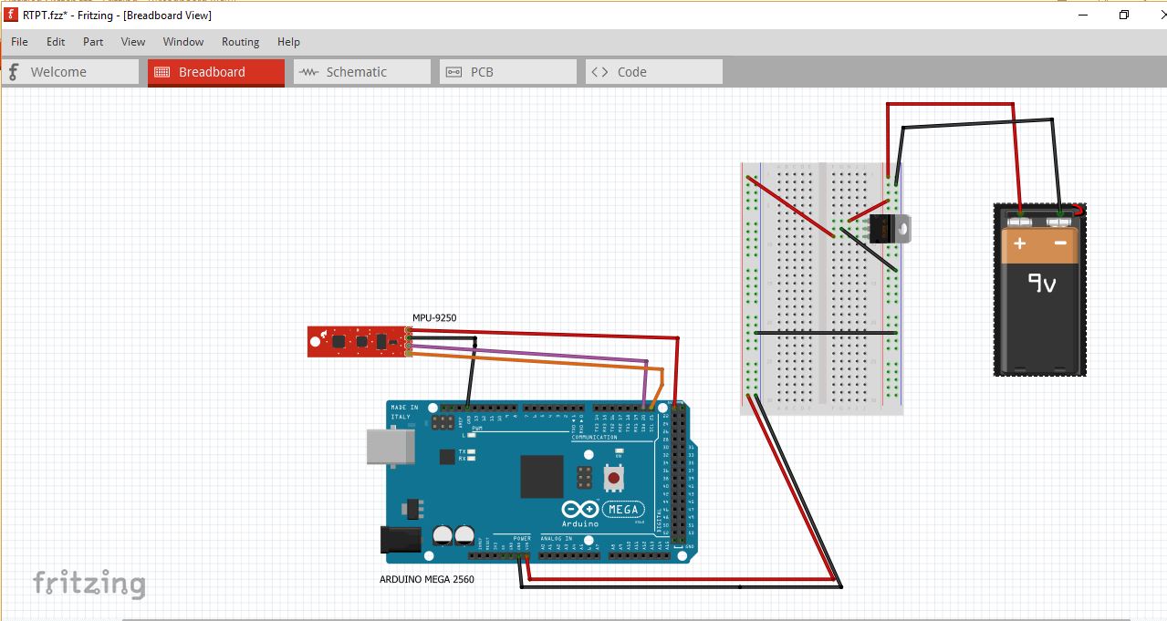
Once you save the library to your Arduino folder you are ready to go. Open the example MPU9250BasicAHRS.ino. Also have this setup ready:
MPU9250 Breakout ——— Arduino
- VIN ———————- 5V
- SDA ———————– SDA (Pin 20)
- SCL ———————– SCL (Pin 21)
- GND ———————- GND
These wires shouldn't be very long because I2C connections don't work well for long wires.
Now clean up the MPU9250BasicAHRS code. It has LCD code in it, but we don't need it, so remove unnecessary lines. Also I have added a part of auto calibration code. Here is the modified code without unnecessary code and added auto calibration: Github.
Now upload the code to your Arduino and make the connections shown above. Open the Serial Terminal and change the baud rate to 115200. You should see this output:
MPU9250
9-DOF 16-bit
motion sensor
60 ug LSB
MPU9250 I AM 71 I should be 71
MPU9250 is online…
x-axis self test: acceleration trim within : 0.8% of factory value
y-axis self test: acceleration trim within : -1.9% of factory value
z-axis self test: acceleration trim within : 1.8% of factory value
x-axis self test: gyration trim within : -0.2% of factory value
y-axis self test: gyration trim within : 0.3% of factory value
z-axis self test: gyration trim within : 0.6% of factory value
MPU9250 bias
x   y   z
254913-660mg1.1-0.11.2o/s
MPU9250 initialized for active data mode….
AK8963 I AM 48 I should be 48
AK8963 initialized for active data mode….
Mag Calibration: Wave device in a figure eight until done!
If you see this:
MPU9250
9-DOF 16-bit
motion sensor
60 ug LSB
MPU9250 I AM FF I should be 71
Could not connect to MPU9250: 0xFF
This means there is definitely a wiring problem (or in the worst case Mpu/arduino fault) try to rectify it before proceeding.
If everything goes well and you see “MPU is online” and “Mag Calibration: Wave device in a figure eight until done!” then everything is working and you should wave your mpu in figure eights until it finishes the auto calibration. After a while you should be getting yaw, pitch, and roll output as below:
Mag Calibration: Wave device in a figure eight until done!
Mag Calibration done!
X-Axis sensitivity adjustment value 1.19
Y-Axis sensitivity adjustment value 1.19
Z-Axis sensitivity adjustment value 1.15
AK8963
ASAX
1.19
ASAY
1.19
ASAZ
1.15
Yaw, Pitch, Roll: 11.34, 28.62, 50.03
Yaw, Pitch, Roll: 20.47, 25.15, 52.88
Yaw, Pitch, Roll: 26.94, 19.02, 52.70
Yaw, Pitch, Roll: 28.22, 15.02, 50.15
Yaw, Pitch, Roll: 27.10, 13.94, 44.68
Yaw, Pitch, Roll: 23.11, 13.69, 37.51
Yaw, Pitch, Roll: 14.29, 13.22, 27.61
Yaw, Pitch, Roll: 357.03, 8.21, 16.72
Yaw, Pitch, Roll: 342.29, 0.69, 9.19
Yaw, Pitch, Roll: 328.42, -4.80, 3.16
Yaw, Pitch, Roll: 317.19, -10.51, -0.58
Yaw, Pitch, Roll: 311.88, -16.57, -3.64
Yaw, Pitch, Roll: 327.71, -23.45, -16.82
Yaw, Pitch, Roll: 325.74, -22.02, -23.51
Yaw, Pitch, Roll: 325.99, -28.17, -26.95
Yaw, Pitch, Roll: 324.57, -24.96, -23.21
Yaw, Pitch, Roll: 320.01, -26.42, -22.25
Yaw, Pitch, Roll: 322.50, -26.04, -26.62
Yaw, Pitch, Roll: 322.85, -23.43, -29.17
Yaw, Pitch, Roll: 323.46, -19.20, -31.48
Awesome! Now you have the data, and you can play with real time motion!😀
Auto Azimuth (Yaw) calibration of RTPT using P- controllerWe first convert yaw from (-180 to +180) to (0 to 360) by doing:
yaw = yaw + 180;Then we just find the error in yaw using a simple Proportional controller and then add the error back to yaw and then do the servo mappings with the new yaw:
nyaw = 360 – yaw;      //”yaw” comes from MPU which is “actual”
Azim = Azimuth – nyaw;         /*”Azimuth” is the absolute azimuth which  comes    from  calculations from RA and DEC   which assumes our device is already aligned to    North….by doing the subtraction we get the proportional error*/
Azim -= 90;        //adding 90° because my titlt servo is mounted at an offset of 90°
while (Azim < 0)
Azim = 360.0 – abs(Azim);     /*we use the error proportionally for our servo to auto adjust */
Azi = map(Azim, 0, 360, 5, 29);
Az = (int)Azi;
Elev = map(Elevation, -90, 90, 2, 178);
El = (int)Elev;
This completes my RTPT project. Hope you have learned new things from it. 🙂
The final code is in the main RTPT page.
Thank you!😀


_3u05Tpwasz.png?auto=compress%2Cformat&w=40&h=40&fit=fillmax&bg=fff&dpr=2)
Comments