


We are a team of nine undergraduate students from a variety of backgrounds (chemistry, physics, biology, chemical engineering and medical engineering), but with a shared interest in biophysics. We were initially brought together by our supervisor, who researches bioreactors for wastewater purification to look at the role of quantum mechanics in biology.
Our project so far has been focussed on reading and finding topics for us to research that are linked, but also are tied to our specialties. We were inspired by the potential of microbial fuel cells and bioreactors as a source of energy and wanted to look further into exoelectrogenic Geobacter to understand how it transfers electrons to other species and electrodes.
We have now split into subteams and are working on:
- structure of proteins involved in extracellular electron transfer eg. cytochrome
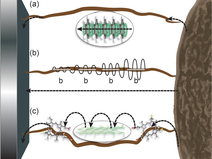
- quantum mechanics of electron transport in these proteins using tunnelling, hopping and superexchange
- roles of hydroquinones in electron transfer across the inner cell membrane of Geobacter
- effect of surface topography on adhesion of bacteria to surfaces (for potential application in bioreactors and fuel cells)
- formation of biofilm and communication between bacteria (can be applied to fuel cells where bacteria form a film on the electrode
Free energy of adhesion to a surface with cavities
Python# -*- coding: utf-8 -*-
"""
Final script - combines all the parts to reproduce work of Zhao et al., ‘A New Method for Modeling Rough Membrane Surface and Calculation of Interfacial Interactions’. with constants altered for GAC Geobacter system. Contains code from part2 and part 5a.
Created on Fri Jul 19 15:26:34 2019
@author: Hannah Sanderson
"""
#Step 1 calculate surface energies per unit area and input required parameters
import math
import numpy as np
#define constants, for source of values see 'Bigscript1 constant values.docx'
I=0.01 # I is molarity of electrolyte, based on data from Henry
h0=0.158e-9 #minimum equilibrium cut-off distance
eps0=8.854e-12 #permittivity of free space
epsr=79 #static relative permittivity of water
k=3.28e9*math.sqrt(I) #Debye screening length
l=0.6e-9 #decay length for AB interactions in water
# decide values for surface tensions, see constants document
#mlw, mp, mn are membrane LW and polar surface tension parameters
#wlw, wp, wn; plw, pp, pn are water and particle surfaces (change from f for foulant in Zhao paper)
#all values are in standard SI units
#Geobacter
#plw=47.25e-3
#pp=0.153e-3
#pn=16.95e-3
#pzeta=-27e-3
#M. Barkeri
plw=35.89e-3
pp=2.12e-3
pn=54.11e-3
pzeta=-23e-3
wlw=21.8e-3
wp=25.5e-3
wn=25.5e-3
mlw=39.45e-3
mp=2.86e-3
mn=1.64e-3
mzeta=-40e-3 #adjusting for pH 10
# calculate delta G per unit area at minimum equilibrium cut-off distance
dglw=-2*(math.sqrt(mlw)-math.sqrt(wlw))*(math.sqrt(plw)-math.sqrt(wlw)) #Lifshitz van der Waals
dgab=2*(math.sqrt(wp)*(math.sqrt(pn)+math.sqrt(mn)-math.sqrt(wn))+math.sqrt(wn)*(math.sqrt(pp)+math.sqrt(mp)-math.sqrt(wp))-math.sqrt(pn*mp)+math.sqrt(pp*mn)) #Lewis acid base
def dgel(d): #electrostatic double layer - defined as a function as need expression that varies with d when you integrate
return 0.5*eps0*epsr*k*(pzeta**2+mzeta**2)*(1-(1/math.tanh(k*d))+((2*mzeta*pzeta*(1/math.sinh(k*d)))/(mzeta**2+pzeta**2)))
#Step 2 - perform integration
#expression we want to integrate that appears in all of them
#r*(d+rparticle-math.sqrt(rparticle**2-r**2)+2*px-z(r,theta)) (extra factor of r due to rdrdtheta surface element)
#integrate excluding the first term and just add pi*rparticle**2 to result
#this makes the code run faster
from scipy import integrate
#import your desired surface - change script_name and where you import from, do not change what you import as, may need to change plot section for some scripts
import flattened_cavity_on_axis as ds
script_name=input('What should we call these files?\n')
#define particle radius
rparticle=1e-6 #correct order of magnitude size of geobacter and 100 times greater than surface seperation so formulae still hold
# superfluous code plot the surface so you can see what you've made, can remove here to :-) if desired
rin=1e-6 #choose radius of your displayed plot to be at least as big as rparticle
R=np.linspace(0,rin, 50)
Theta=np.linspace(0, 2*math.pi, 50)
rplot,thetaplot=np.meshgrid(R,Theta) #makes a grid of r, theta points
x=rplot*np.cos(thetaplot) #makes x-y grid for plot
y=rplot*np.sin(thetaplot)
zplot=ds.depth-ds.z(rplot,thetaplot) #need to modify this line to d-ds.z for parabola due to how surface is defined
from mpl_toolkits.mplot3d import Axes3D
import matplotlib.pyplot as plt
from matplotlib.ticker import FormatStrFormatter
fig = plt.figure()
ax = fig.gca(projection='3d')
surf=ax.plot_surface(x,y,zplot,cmap='afmhot') #label surface so can use it later
ax.xaxis.set_major_locator(plt.MaxNLocator(5))
ax.xaxis.set_major_formatter(FormatStrFormatter('%.1e'))
ax.yaxis.set_major_locator(plt.MaxNLocator(5))
ax.yaxis.set_major_formatter(FormatStrFormatter('%.1e'))
ax.set_zticklabels([]) #hide z axis labels as makes plot too cluttered
#label axes
plt.title(script_name)
plt.xlabel('x/m')
plt.ylabel('y/m')
plt.colorbar(surf) #label z axis with colorbar instead
ax.set_zlabel('height/m') #difference in syntax here for 3d plot not sure about this maybe change later for consistency
plt.savefig(script_name+' surface_plot.png',dpi=1200)
# :-)
#required code restarts here
#define function to integrate - n.b. this is different from big script 1 as z(r,theta) is defined differently so no longer need surface amplitude
def integ(r,theta):
return r*(rparticle-math.sqrt(rparticle**2-r**2)+ds.z(r,theta))
# perform integration - remember this will return a value and an error!
result=integrate.dblquad(integ,0,2*math.pi,0,rparticle)
#Step 3 - add distance dependence
#define kT energy scaling factor - choose room temperature
kT=1.38e-23*293
def Ulw(d): #Lifshitz van der Waals
return dglw*(h0**2/d**2)*(result[0]+(rparticle**2)*d*math.pi)/kT
def Uab(d): #Lewis acid-base
return dgab*math.e**((h0-d)/l)*(result[0]+(rparticle**2)*d*math.pi)/kT
d=np.linspace(1e-9,15e-9,1000) #can choose range and how many points, don't go closer than 1nm as plots tend to infinity and it ruins scaling
def Uel(d): #electrostatic double layer - need to define as a function as is more complicated, for each d define a new value for Uel output
i=0
Uelout=np.zeros(len(d))
while i<len(d):
din=d[i]
Uelout[i]=dgel(din)*(result[0]+(rparticle**2)*din*math.pi)/kT
i=i+1
return Uelout
def Utot(d): #total interaction energy
return Uel(d)+Uab(d)+Ulw(d)
#define array of total interaction energies to find barrier height
utot=Utot(d)
x=max(utot)
xlab=format(x,'.2e')
locmax=np.argmax(utot)
#this Uel has same shape as in paper for this molarity, but does have a turning oint at 0.5e-9, however this is not shown in the paper, this could also be where
#the electrostatic model breaks down if the seperation is too small, so maybe the turning point is not there in reality, but goes off to infinity
#Step 4: plot graphs as a function of d
import matplotlib.pyplot as plt
plt.figure()
plt.subplot(3,1,1) #could spend more time on the axis scaling later if desired
plt.title('Interaction energies a function of distance for a \n'+script_name)
plt.plot(d,Ulw(d))
plt.ylabel('$U_{LW}(d)$/kT')
plt.xlabel('d/nm')
plt.subplot(3,1,2)
plt.plot(d,Uab(d))
plt.ylabel('$U_{AB}(d)$/kT')
plt.xlabel('d/nm')
plt.subplot(3,1,3)
plt.plot(d,Uel(d))
plt.ylabel('$U_{EL}(d)$/kT')
plt.xlabel('d/nm')
plt.tight_layout(2) #spreads out subplots
plt.autoscale(True,axis='both')
plt.savefig(script_name+' subplot.png',dpi=1200) #modify this with the path where you want to save your files, otherwise will save in same folder as script
fig=plt.figure()
ax=plt.axes()
plt.title('Interaction energies a function of distance for a \n'+script_name)
line1=plt.plot(d,Utot(d),label='Total Interaction Energy')
line2=plt.plot(d,Uel(d),label='$U_{EL}(d)$')
line3=plt.plot(d,Uab(d),label='$U_{AB}(d)$')
line4=plt.plot(d,Ulw(d),label='$U_{LW}(d)$')
plt.axhline(y=0,color='k',linestyle='--') #adds horizontal, dashed line at y=0
plt.legend() #legend labels automatically with labels you assigned to your lines
plt.ylabel('Iteraction energy/kT')
plt.ylim([-1.4*x,1.4*x]) # scaled by height of energy barrier so energy barrier is always displayed on the plot
plt.xlabel('d/m')
plt.xlim([0,15e-9])#alter depending on d input - currently up to 15nm
ax.text(d[locmax],max(utot),xlab)
plt.savefig(script_name+' total_plot.png',dpi=1200)
print(d[locmax])
print(xlab)
print('Hip hip hooray')
Flattened cavity model
Python# -*- coding: utf-8 -*-
"""
y=x^16 flattened cavity on axis
Created on Wed Jul 31 16:37:37 2019
@author: Hannah
"""
#define depth (d) and radius of cavity (rcav) in order to get correct scaling
depth=12e-6
rcav=6e-6
c=depth/(rcav**16)
#define function
def z(r,theta):
return depth-c*(r**16) #defined by subtracting curve off cavity depth
Free energy of adhesion to a rough surface
Python# -*- coding: utf-8 -*-
"""
Final script - combines all the parts to reproduce work of Zhao et al., ‘A New Method for Modeling Rough Membrane Surface and Calculation of Interfacial Interactions’. with constants altered for GAC Geobacter system.
Created on Fri Jul 19 15:26:34 2019
@author: Hannah Sanderson
"""
#Step 1 calculate surface energies per unit area and input required parameters
import math
import numpy as np
#define constants, for source of values see 'Bigscript1 constant values.docx'
I=0.01 # I is molarity of electrolyte, based on data from Henry
h0=0.158e-9 #minimum equilibrium cut-off distance
eps0=8.854e-12 #permittivity of free space
epsr=79 #static relative permittivity of water
k=3.28e9*math.sqrt(I) #Debye screening length
l=0.6e-9 #decay length for AB interactions in water
# decide values for surface tensions, see constants document
#mlw, mp, mn are membrane LW and polar surface tension parameters
#wlw, wp, wn; plw, pp, pn are water and particle surfaces (change from f for foulant in Zhao paper)
#all values are in standard SI units
#Geobacter
#plw=47.25e-3
#pp=0.153e-3
#pn=16.95e-3
#pzeta=-27e-3
wlw=21.8e-3
wp=25.5e-3
wn=25.5e-3
mlw=39.45e-3
mp=2.86e-3
mn=1.64e-3
mzeta=-40e-3 #adjusting for pH 10
#M. Barkeri
plw=35.89e-3
pp=2.12e-3
pn=54.11e-3
pzeta=-23e-3
# calculate delta G per unit area at minimum equilibrium cut-off distance
dglw=-2*(math.sqrt(mlw)-math.sqrt(wlw))*(math.sqrt(plw)-math.sqrt(wlw)) #Lifshitz van der Waals
dgab=2*(math.sqrt(wp)*(math.sqrt(pn)+math.sqrt(mn)-math.sqrt(wn))+math.sqrt(wn)*(math.sqrt(pp)+math.sqrt(mp)-math.sqrt(wp))-math.sqrt(pn*mp)+math.sqrt(pp*mn)) #Lewis acid base
def dgel(d): #electrostatic double layer - defined as a function as need expression that varies with d when you integrate
return 0.5*eps0*epsr*k*(pzeta**2+mzeta**2)*(1-(1/math.tanh(k*d))+((2*mzeta*pzeta*(1/math.sinh(k*d)))/(mzeta**2+pzeta**2)))
#Step 2 - perform integration
#expression we want to integrate that appears in all of them
#r*(d+rparticle-math.sqrt(rparticle**2-r**2)+2*px-z(r,theta)) (extra factor of r due to rdrdtheta surface element)
#integrate excluding the first term and just add pi*rparticle**2 to result
#this makes the code run faster
from scipy import integrate
#import your desired surface - change script_name and where you import from, do not change what you import as, may need to change plot section for some scripts
import sinusoidal_surface as ds
script_name=input(str('What do you want to call these files?\n'))
#define particle radius
rparticle=1e-6 #correct order of magnitude size of geobacter and 100 times greater than surface seperation so formulae still hold
# superfluous code plot the surface so you can see what you've made, can remove here to :-) if desired
rin=1e-6 #choose radius of your displayed plot to be at least as big as rparticle
R=np.linspace(0,rin, 50)
Theta=np.linspace(0, 2*math.pi, 50)
rplot,thetaplot=np.meshgrid(R,Theta) #makes a grid of r, theta points
x=rplot*np.cos(thetaplot) #makes x-y grid for plot
y=rplot*np.sin(thetaplot)
zplot=ds.z(rplot,thetaplot) #need to modify this line to d-ds.z for parabola due to how surface is defined
from mpl_toolkits.mplot3d import Axes3D
import matplotlib.pyplot as plt
from matplotlib.ticker import FormatStrFormatter
fig = plt.figure()
ax = fig.gca(projection='3d')
surf=ax.plot_surface(x,y,zplot,cmap='RdBu') #label surface so can use it later
ax.xaxis.set_major_locator(plt.MaxNLocator(5))
ax.xaxis.set_major_formatter(FormatStrFormatter('%.1e'))
ax.yaxis.set_major_locator(plt.MaxNLocator(5))
ax.yaxis.set_major_formatter(FormatStrFormatter('%.1e'))
ax.set_zticklabels([]) #hide z axis labels as makes plot too cluttered
#label axes
plt.title(script_name)
plt.xlabel('x/m')
plt.ylabel('y/m')
plt.colorbar(surf) #label z axis with colorbar instead
ax.set_zlabel('height/m')
plt.savefig(script_name+'surface_plot.png',dpi=1200)
# :-)
#required code restarts here
#define function to integrate - n.b. this is different from big script 1 as z(r,theta) is defined differently so no longer need surface amplitude
def integ(r,theta):
return r*(rparticle-math.sqrt(rparticle**2-r**2)+2*ds.px-ds.z(r,theta))
# perform integration - remember this will return a value and an error!
result=integrate.dblquad(integ,0,2*math.pi,0,rparticle)
#Step 3 - add distance dependence
#define kT energy scaling factor - choose room temperature
kT=1.38e-23*293
def Ulw(d): #Lifshitz van der Waals
return dglw*(h0**2/d**2)*(result[0]+(rparticle**2)*d*math.pi)/kT
def Uab(d): #Lewis acid-base
return dgab*math.e**((h0-d)/l)*(result[0]+(rparticle**2)*d*math.pi)/kT
d=np.linspace(1e-9,15e-9,1000) #can choose range and how many points, don't go closer than 1nm as plots tend to infinity and it ruins scaling
def Uel(d): #electrostatic double layer - need to define as a function as is more complicated, for each d define a new value for Uel output
i=0
Uelout=np.zeros(len(d))
while i<len(d):
din=d[i]
Uelout[i]=dgel(din)*(result[0]+(rparticle**2)*din*math.pi)/kT
i=i+1
return Uelout
def Utot(d): #total interaction energy
return Uel(d)+Uab(d)+Ulw(d)
#define array of total interaction energies to find barrier height
utot=Utot(d)
x=max(utot)
xlab=format(x,'.2e')
locmax=np.argmax(utot)
#this Uel has same shape as in paper for this molarity, but does have a turning oint at 0.5e-9, however this is not shown in the paper, this could also be where
#the electrostatic model breaks down if the seperation is too small, so maybe the turning point is not there in reality, but goes off to infinity
#Step 4: plot graphs as a function of d
import matplotlib.pyplot as plt
plt.figure()
plt.subplot(3,1,1) #could spend more time on the axis scaling later if desired
plt.suptitle('Interaction energies a function of distance for a\n '+script_name)
plt.plot(d,Ulw(d))
plt.ylabel('$U_{LW}(d)$/kT')
plt.xlabel('d/nm')
plt.subplot(3,1,2)
plt.plot(d,Uab(d))
plt.ylabel('$U_{AB}(d)$/kT')
plt.xlabel('d/nm')
plt.subplot(3,1,3)
plt.plot(d,Uel(d))
plt.ylabel('$U_{EL}(d)$/kT')
plt.xlabel('d/nm')
plt.tight_layout(2) #spreads out subplots
plt.autoscale(True,axis='both')
plt.savefig(script_name+'subplot.png',dpi=1200) #modify this with the path where you want to save your files, otherwise will save in same folder as script
fig=plt.figure()
ax=plt.axes()
plt.title('Interaction energies a function of distance for a \n'+script_name)
line1=plt.plot(d,Utot(d),label='Total Interaction Energy')
line2=plt.plot(d,Uel(d),label='$U_{EL}(d)$')
line3=plt.plot(d,Uab(d),label='$U_{AB}(d)$')
line4=plt.plot(d,Ulw(d),label='$U_{LW}(d)$')
plt.axhline(y=0,color='k',linestyle='--') #adds horizontal, dashed line at y=0
plt.legend() #legend labels automatically with labels you assigned to your lines
plt.ylabel('Iteraction energy/kT')
plt.ylim([-1.4*x,1.4*x]) # scaled by height of energy barrier so energy barrier is always displayed on the plot
plt.xlabel('d/m')
plt.xlim([0,15e-9])#alter depending on d input - currently up to 15nm
ax.text(d[locmax],max(utot),xlab)
plt.savefig(script_name+' total_plot.png',dpi=1200)
print(d[locmax])
print('et voila!')
sinusoidal_surface
Python# -*- coding: utf-8 -*-
"""
sinusoidal surface
Created on Fri Jul 26 12:00:42 2019
@author: Hannah Sanderson
"""
import numpy as np
import math
depth=160e-9
width=160e-9
#define surface and particle radius
px=depth/2 #amplitude
py=px
wx=width*2 #period
wy=width*2
rparticle=1e-6 #correct order of magnitude size of geobacter and 100 times greater than surface seperation so formulae still hold
def z(r,theta): #define z as a function to enable integration - this will change for different surfaces
return px*np.cos(math.pi*r*np.cos(theta)/(2*wx))+py*np.cos(math.pi*r*np.sin(theta)/(2*wy))


Comments